GRPO is just PPO for bandits

DeepSeek-R1 [1] is the first open-source model that exhibits comparable performance to closed source LLMs, by utilizing Reinforcement learning (RL) to improve reasoning ability after the Supervised Fine-Tuning (SFT) stage.

In a precursory LLM model named DeepSeekMath [2], the team introduced their RL method tagged Group Relative Policy Optimization (GRPO), which is a variant of Proximal Policy Optimization (PPO) [3].

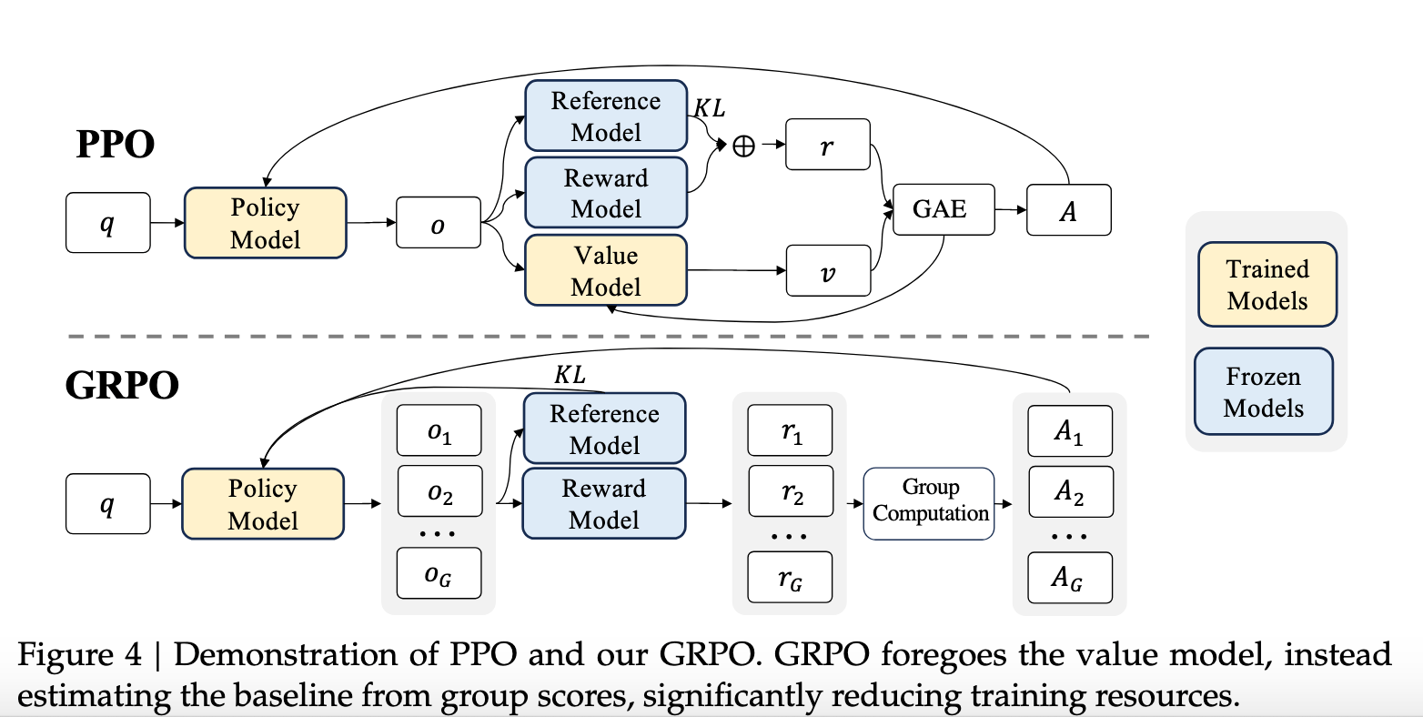
This method is similar to PPO, and optimizes the memory usage by not relying on a learned value function approximation, which would be expensive in memory to maintain. It uses instead the average reward of multiple sampled outputs, produced in response to the same question, as the baseline. More specifically, for each question [math]q[/math], GRPO samples a group of outputs [math]\{o_1, o_2,\ldots, o_G\}[/math] from the old policy [math]\pi_{\theta_{old}}[/math], maps them to rewards [math]\{r_1, r_2,\ldots, r_G\}[/math] using a (possibly parameterized) reward function [math]r_i=r_{\phi}(o_i)[/math] and then optimizes the policy model by maximizing the following objective:

[math] \begin{align}J_{GRPO}(\theta) = \mathbb{E}_{[q\sim P(Q), \{o_i\}_{i=1}^G\sim \pi_{\theta_{old}}(O|q)]} \frac{1}{G}\sum_{i=1}^G \{f(\rho_{\theta},\hat{A}_i)-\beta D_{KL}[\pi_{\theta}||\pi_{ref}]\}\end{align}[/math]

The above objective is in expectation over the distribution of questions [math]P(Q)[/math] and the old policy [math]\pi_{\theta_{old}}[/math]. The function [math]f[/math] is the clipping formula using advantages [math]\hat{A}_i[/math]

[math]f(\rho_{\theta},\hat{A}_i) = \min\left[\rho_{\theta}\hat{A}_{i},clip(\rho_{\theta},1-\epsilon,1+\epsilon)\hat{A}_{i}\right][/math].

In the above expression, the policy ratios are defined as

[math]\begin{align}\rho_{\theta} = \frac{\pi_{\theta}(o_{i}|q)}{\pi_{\theta_{old}}(o_{i}|q)}\end{align}[/math],

and the advantage is defined using only the rewards from collected observations

[math]\begin{align} \hat{A}_i=\frac{r_i-mean(r_1,\ldots,r_G)}{std(r_1,\ldots,r_G)}\end{align}[/math].

Furthermore, the Kullback-Leibler (KL) divergence in the expression aims to keep the policy [math]\pi_{\theta}[/math] as close as possible to the SFT initial phase [math]\pi_{ref}[/math]. It actually uses an unbiased estimator [4] from each sample of question-answer [math](q,o_i)[/math]

[math]\begin{align}D_{KL}[\pi_{\theta}||\pi_{ref}]\} \approx \frac{\pi_{ref}(o_i|q)}{\pi_{\theta}(o_i|q)}- \log\frac{\pi_{ref}(o_i|q)}{\pi_{\theta}(o_i|q)} – 1\end{align}[/math].

An intuitive presentation of GRPO is presented in [5].

Here we present a simple way to derive the GRPO step by step using its building blocks. Essentially we will show that GRPO is a policy gradient method for immediate rewards, similar to bandit algorithms.

Step 1: Policy gradient for one-step rewards

The GRPO as so many other RL algorithms aims to find a policy [math]\pi_{\theta^*}[/math] to maximize the expected reward. The randomness is from the environment, i.e. the person asking the question, as well as the learned policy which can be probabilistic. Here, someone is asking a question [math]q[/math] following some distribution [math]P(q)[/math]. The objective to be maximized is

[math]\begin{align}J(\theta) = \mathbb{E}_{\pi_{\theta}}[r_{t_0}+\gamma r_{t_1}+\gamma^2 r_{t_2}+\ldots] \stackrel{\gamma=0}{\rightarrow}\mathbb{E}_{\pi_{\theta}}[r_{t_0}]= \sum_{q\in Q}d(q)\sum_{o\in O}\pi_{\theta}(o|q)r(o,q) \end{align}[/math],

where [math]d(q)[/math] is the frequency of requesting question [math]q[/math]. In the single hop (bandit) case, where the discount factor is zero, one can realize that there is no need to refer to the Policy Gradient Theorem [9] because the only dependence on [math]\theta[/math] is on the policy and not on some value function because only the immediate reward counts. Then we write

[math]\begin{align}\nabla_{\theta}J(\theta) = \sum_{q\in Q}d(q)\sum_{o\in O}r(o,q)\nabla_{\theta}\pi_{\theta}(o|q) = \mathbb{E}_{q\sim P(q), o\sim \pi_{\theta}}\left[r(o,q)\nabla_{\theta}\log(\pi_{\theta}(o|q))\right]\end{align}[/math].

Note that we can use the empirical average to approximate the expectation over the policy output. As GRPO claims, we sample [math]\{o_1,\ldots,o_G\}[/math] answers for the question q, using our current formula, and approximate the above gradient by the empirical one

[math]\begin{align}\nabla_{\theta}J(\theta) \approx \mathbb{E}_{q\sim P(q), \{o_1,\ldots,o_G\}\sim \pi_{\theta}}\frac{1}{G}\sum_{i=1}^G\left(r(o_i,q)\nabla_{\theta}\log(\pi_{\theta}(o_i|q))\right)\end{align}[/math].

Step 2: Generalized Advantage

In the above, the immediate reward [math]r(o,q)[/math] takes the place of the state-action value function [math]Q_{\theta}(o,q)[/math] of the standard policy gradient. From [6], it is very usual to replace in the policy gradient the state-action value function by the advantage [math]A(o,q)= Q_{\theta}(o,q)-V(s)[/math]. In practice [7], instead of subtracting from each [math]Q_{\theta}(o,q)[/math] the maximum value function among all possible answers [math]\max_o Q_{\theta}(o,q)[/math] we can also subtract the average over all possible actions from the set [math]O[/math]

[math]\begin{align}A(o,q)= Q_{\theta}(o,q)-\frac{1}{|O|}\sum_{i=1}^O Q_{\theta}(o_i,q)\stackrel{\gamma=0}{\rightarrow} A(o,q)= r(o,q)-\frac{1}{|O|}\sum_{i=1}^O r(o_i,q)\end{align}[/math].

Since we cannot have the entire range of answers available, we use here in the GRPO the available answers [math]\{o_1,\ldots,o_G\}[/math] only. Combining the above two steps we would like to maximize the following objective

[math]\begin{align}\max_{\theta} \ L^{Policy Gradient}(\theta) = \mathbb{E}_{q\sim P(q), o\sim\pi_{\theta}}\left[A(o,q)\log(\pi_{\theta}(o|q))\right]\end{align}[/math].

Step 3: TRPO

In the TRPO paper [8] the above objective is replaced by a surrogate objective

[math]\begin{align}\max_{\theta} \ L^{TRPO}(\theta) = \mathbb{E}_{q\sim P(q), o\sim\pi_{\theta_{old}}}\left[A_{old}(o,q)\frac{\pi_{\theta}(o|q)}{\pi_{\theta_{old}}(o|q)})\right]\end{align}[/math].

We consider the policy is updated step-wise. Once we have some version [math]\pi_{\theta_{old}}(o|q)[/math] we collect observations [math]\{o_1,\ldots,o_G\}[/math], calculate the advantages and plug this information in the above formula to update the policy. From an intuitive point of view, [math]L^{TRPO}(\theta)[/math] and [math]L^{Policy Gradient}(\theta)[/math] are very similar to each other. Remember that the derivative of the latter is

[math]\begin{align}\mathbb{E}[A(o,q)\nabla\log{\pi_{\theta}(o|q)}] = \mathbb{E}\left[A(o,q)\frac{\nabla\pi_{\theta}(o|q)}{\pi_{\theta}(o|q)}\right]\stackrel{freeze\theta_{old}}{=} \mathbb{E}\left[A_{old}(o,q)\frac{\nabla\pi_{\theta}(o|q)}{\pi_{\theta_{old}}(o|q)}\right] \end{align}[/math]

Then, obviously the right-hand side is just the derivative of [math]L^{TRPO}(\theta)[/math].

Step 4: PPO

The PPO paper introduces the clipped surrogate objective function [math]f(\rho_{\theta},\hat{A}_i) = \min\left[\rho_{\theta}\hat{A}_{i},clip(\rho_{\theta},1-\epsilon,1+\epsilon)\hat{A}_{i}\right][/math] that we saw above in the GRPO, in order to bound the steps of the new policy update compared to the old policy. The aim is to keep the next update close to the previous one. If the advantage is positive and the new policy favors this compared to the old policy then the function clips above to [math]1+\epsilon[/math] how much the improvement can allowed to be. In the case of negative advantage, if the new policy defavorizes it, then the reduction is clipped below by [math]1-\epsilon[/math].

Finally, the Kullback-Leibler divergence of the new policy compared to the reference one, further limits the update step to keep it close to SFT which has been trained on acceptable and desirable outcomes.

Conclusion

It is important to observe that the PPO value function estimation was never necessary in the first place. The question-answer problem is one-hop and hence similar to the bandit problems. This was already mentioned in the paper [10]: “The environment is a bandit environment which presents a random customer prompt and expects a response to the prompt. Given the prompt and response, it produces a reward determined by the reward model and ends the episode.”

Consequently, the importance in the GRPO lies in the relation between the reward mapping [math]r_{\phi}(o)[/math], the policy-gradient, and how many samples G can be collected (which in LLMs is expensive). Also, rather important seems to be the answer sampling policy. Such a discussion and the sensitivity of the outcome with respect to the design of the reward function has been shown in the very nice analysis by Marc Lelarge in his GitHub page [11].

Realizing that GRPO is just a sophisticated bandit algorithm, maybe other methods in the future can establish as good or better convergence. On the other hand, there could be interest to study how a sequence of questions-answers can be trained using classic PPO, maybe producing more interesting tuning since it will account for chain of interactions, instead of single-hop.

@article{giovanidis2025_GRPO,
title = “GRPO is just PPO for Bandits”,
author = “Giovanidis, Anastasios”,
journal = “anastasiosgiovanidis.net”,
year = “2025”,
url = “https://anastasiosgiovanidis.net/2025/02/17/grpo-is-just-ppo-for-bandits/“
}

References

[9] Sutton et al. “Policy Gradient Methods for Reinforcement Learning with Function Approximation“, NeurIPS 1999

[10] Ouyang et al. “Training language models to follow instructions with human feedback”, arXiv:2203.02155v1

[11] https://github.com/dataflowr/notebooks/blob/master/llm/Gauss_GRPO.ipynb