Category Archives: Uncategorized

When Everyone Asks the Same Machine

How shared AI inspiration could reshape human creativity – and the machines that learn from it.

Published: September 2026 • Reading time: 9 min

Imagine the Web twenty years from now.

A researcher asks an LLM to help write a paper. An engineer asks one to prepare documentation. A student uses one to answer a question. A journalist uses one to structure an article. A programmer asks one to explain a bug. None of them simply copies what the machine produces. They read it, correct it, argue with it, perhaps rewrite half of it. The resulting material may be excellent. But it does not disappear when they are finished with it. It becomes part of the Web: Tomorrow’s papers, documentation, tutorials, articles and discussions. And some of that material will eventually help train the next generation of machines. Now multiply this process by hundreds of millions of people. We are beginning to create a loop:

human knowledge→AI→human–AI content→future AI.\text{human knowledge} \rightarrow \text{AI} \rightarrow \text{human–AI content} \rightarrow \text{future AI}.
A scene depicting two humans and two robots painting on easels in a well-lit studio. The humans are focused on colorful abstract compositions, while the robots replicate realistic still life images of vases and bowls.

There is nothing necessarily alarming about this. Human culture has always been recursive. We read other people, absorb their ideas and write new things. Scientists build on earlier scientists. Writers imitate writers before finding their own voices. But generative AI changes the scale – and perhaps the structure – of that recursion.

The first generation of large language models inherited something historically extraordinary: an enormous corpus produced mostly without large language models. Scientists wrote papers. Programmers argued late into the night on forums. Someone maintained a webpage devoted to an obscure radio receiver. Students asked questions that experts would never have thought to ask. Journalists interviewed people whose experiences existed nowhere else. Hobbyists documented failed experiments. People wrote beautifully and badly, carefully and impulsively. They disagreed, misunderstood each other, invented terminology and approached the same problems from different directions. The Web was noisy, repetitive and frequently wrong. But its messiness contained something precious: diversity of origin.

What happens when an increasing fraction of that diversity passes through the same generative machinery?

This is no longer an entirely hypothetical concern. Recent experiments have found that AI-assisted or AI-generated creative work can become more homogeneous at the collective level. In one study of 2,200 college-admissions essays, each additional human-written essay contributed more new ideas to the collective pool than an additional GPT-4 essay. Remarkably, increasing the diversity of individual AI outputs did not eliminate the gap in collective diversity.[1] A recent meta-analysis covering 19 studies and 61 effect sizes reaches a more cautious but similar conclusion: generative AI is associated with a small but significant homogenization effect in human–AI co-creation, although the magnitude depends on the task and on how people interact with the system.[2]

The danger, then, is not necessarily that AI-generated information becomes bad. Something subtler can happen:

individual quality↑collective diversity↓.\text{individual quality}\uparrow \qquad \text{collective diversity}\downarrow.

An Information-Theoretic Limit

Information theory has a wonderfully unforgiving principle for what happens when information is repeatedly processed. Suppose information passes through a sequence

X→Y→Z.X\rightarrow Y\rightarrow Z.

If Z receives its information about X only through Y, the Data Processing Inequality tells us that

I(X;Z)≤I(X;Y).I(X;Z)\leq I(X;Y).

In plain language: processing can reorganize information, compress it, reveal patterns in it and make it vastly more useful. But it cannot recreate distinctions about the original source that have already been lost along the way. The principle grew out of the information-theoretic framework established by Claude Shannon and is now one of the field’s basic results. Cover and Thomas give its standard treatment in Elements of Information Theory.[3]

Now imagine an idealized chain:

H→M0→S1→M1→S2→⋯H\rightarrow M_0\rightarrow S_1\rightarrow M_1\rightarrow S_2\rightarrow\cdots

Here H is our accumulated human corpus, M_t a generation of models and S_t the material those models help us produce. This is an analogy, not a literal Markov chain. AI can produce genuinely new results. A mathematical system can derive a proof nobody has previously written down. A model can discover an algorithm, find a surprising strategy or combine known ideas into something its creators had never considered. Nothing in the Data Processing Inequality says otherwise. But the inequality suggests a different question:

When information repeatedly passes through similar representations, which distinctions survive, and which quietly disappear?

That question becomes more interesting once the loop closes. Research on so-called model collapse has already demonstrated one version of the problem inside machine learning. When models are recursively trained on model-generated data, information about the tails of the original distribution can progressively disappear.[4]

The human–AI ecosystem is vastly richer than that experiment. Humans contribute knowledge, judgment and new information at every stage. But this raises the central question of this essay:

Are we injecting enough independent variation back into the loop?

Generative abundance should not be confused with informational diversity.

One Hundred Authors

Imagine a simple experiment. We put one hundred knowledgeable people in one hundred rooms and give them the same difficult question. One person remembers a paper she read ten years ago. Another approaches the problem geometrically because that is how he learned to think. Someone misunderstands the question and, by accident, finds an interesting interpretation of it. One answer is brilliant. Several are pedestrian. A few are simply wrong.

Now repeat the experiment, except this time there is a state-of-the-art language model in every room. Within seconds, each screen fills with an articulate answer. The humans are not passive. They correct mistakes, remove weak arguments and add their own expertise. The second set of answers may well be better. But the hundred authors have acquired a hidden common collaborator. Their texts may still look different, yet their starting points are now more correlated. Similar arguments appear near the top. Similar examples suggest themselves. Some ways of framing the problem are repeatedly offered; others never appear.

A rare idea does not have to be censored to disappear. It only has to stop being suggested.

This is close to what the recent empirical literature is beginning to observe. The effect is not absolute—AI does not make everybody identical—but at scale, shared generative assistance can shift a collection of outputs toward greater similarity.[1,2,5]

And those outputs do not end with their authors. They become papers, webpages, documentation and discussions. Some may eventually enter future training corpora. What was already probable becomes slightly more visible. What was unusual becomes slightly harder to encounter. The loop closes:

model preference→human publication→training corpus→future model preference.\text{model preference} \rightarrow \text{human publication} \rightarrow \text{training corpus} \rightarrow \text{future model preference}.

Correlated Inspiration

There is an obvious objection. Humans have never created from nothing. Music grows from earlier music, mathematics from earlier mathematics, painting from earlier painting. Inspiration is itself a form of inheritance. But historically that inheritance has followed many paths. Different teachers, books, cultures, conversations and accidents shaped different minds. Human culture worked, in a loose sense, like an enormous mixture of experts: overlapping, but never quite seeing the world in the same way.

LLMs were trained on the traces left by this diversity. Now this enormous mixture increasingly turns to the same few models for inspiration. Why should that matter?

Because discovery is partly a search problem.

When many minds approach a question differently, they explore different parts of the space of possible ideas. Most paths lead nowhere. But occasionally the odd path—the one nobody else considered promising—is precisely where something new is found. A common AI assistant can make every explorer individually better while nudging many of them toward the same promising regions.

That creates a paradox: better individual search, but potentially narrower collective exploration.

History occasionally rewards intellectual outliers: an Archimedes or a Leonardo da Vinci, minds that followed unusual combinations of interests and lines of thought. We cannot know whether such figures would have thought differently in an AI-mediated world. That uncertainty is precisely the point. We do not know beforehand which unusual intellectual trajectory will matter.

The value of intellectual diversity is not that every different idea deserves to survive. Most do not. Its value is that we cannot know beforehand which unusual idea, method or question will turn out to matter. The problem is not inspiration.

It is correlated inspiration.

So What Should the Human Do?

The obvious response is more human supervision. That is necessary, but it is not sufficient. A human can carefully verify an AI-generated article while contributing very little outside the model’s original trajectory. We can correct its facts, improve its prose and choose the strongest of five arguments it proposes. That makes us good editors.

But the information ecosystem needs us to be something else as well: sources.

There is a meaningful difference between asking: “Give me five interesting research questions about this problem.”

and arriving with: “Something bothers me about the way we formulate this problem. What happens if we look at it this other way?”

In both cases AI can be enormously useful. But the intellectual direction begins in a different place. In the first case, the model proposes possible directions and the human selects from them. In the second, the human introduces a direction. The machine can then do what it does extraordinarily well: search, challenge the idea, find related work, derive consequences, generate counterexamples and expose weaknesses.

The point is not to keep AI at arm’s length. Quite the opposite. Come to the model with something.

A question. An observation. An objection. A strange analogy. Something you noticed at work. A result that does not fit. An idea that may turn out to be wrong. Then use the machine aggressively. Human–AI interaction does not reduce intellectual diversity simply because AI participates. What matters is whether humans remain active sources within that interaction rather than becoming only selectors of machine-generated possibilities.

To Ask, We Still Need to Learn

There is one catch: to arrive with a good question, we usually need to know something. A researcher questions an assumption because she understands why it was introduced. An engineer notices an anomaly because he knows what normal looks like. We connect two ideas because both were already somewhere in our minds.

Knowledge gives us the landscape against which something can appear surprising.

This is why education cannot simply outsource knowledge to AI. Students still need enough understanding to disagree, wonder and ask their own questions. The objective is not to know everything. It is to know enough to think independently:

knowledge→understanding→questions→new directions.\text{knowledge} \rightarrow \text{understanding} \rightarrow \text{questions} \rightarrow \text{new directions}.

AI can then take those directions much farther than we could alone.

Beyond Russell’s Limit

Bertrand Russell worried about a growing asymmetry: human knowledge expands, while the amount an individual can assimilate remains limited. In a previous essay, The AI Telco Engineer Against Russell’s Limit, I explored what this means in the age of generative AI through the idea of an “audit threshold”: if we cannot personally reproduce everything machines can produce, we must at least understand enough to interrogate and judge it.[6]

There is another side to that argument.

We must also understand enough to remain a source of questions rather than merely a consumer of answers. The answer is not to use AI less. It is to use it actively.

Let machines search farther than we can search, calculate faster than we can calculate and explore more alternatives than we could explore in a lifetime. But preserve enough knowledge and understanding to occasionally look at what the machine gives us and say: No. That is not quite the question I wanted to ask.

Perhaps that small act of intellectual independence will become more valuable, not less, as AI becomes more capable.

The first generation of large language models inherited an extraordinary archive of human intellectual diversity. Our responsibility is not merely to preserve it. It is to make sure that we still have something of our own to add.

References

[1] K. Moon, A. E. Green, and K. Kushlev, “Homogenizing effect of large language models (LLMs) on creative diversity: An empirical comparison of human and ChatGPT writing,” Computers in Human Behavior: Artificial Humans, vol. 6, 100207, 2025.

[2] A. de Rooij and M. M. Biskjaer, “Does generative AI make us think alike? A systematic review and meta-analysis of homogenisation effects in human–AI co-creation,” Behaviour & Information Technology, 2026.

[3] T. M. Cover and J. A. Thomas, Elements of Information Theory, 2nd ed., Wiley, 2006.

[4] I. Shumailov et al., “AI models collapse when trained on recursively generated data,” Nature, vol. 631, pp. 755–759, 2024.

[5] Z. Sourati, A. S. Ziabari, M. Dehghani, “The homogenizing effect of large language models on human expression and thought,” Trends in Cognitive Sciences, 2026.

[6] A. Giovanidis, “The AI Telco Engineer Against Russell’s Limit,” anastasiosgiovanidis.net, 2026.

Cite as

@misc{giovanidis2026dpi,
author = {Anastasios Giovanidis},
title = {When Everyone Asks the Same Machine},
year = {2026},
howpublished = {\url{https://anastasiosgiovanidis.net}},
note = {Online article}
}

Giovanidis, A. (2026). When Everyone Asks the Same Machine. anastasiosgiovanidis.net.

Leave a comment

Filed under Uncategorized

The AI Telco Engineer Against Russell’s Limit

Published: September 2026 • Reading time: 6 min

I have noticed an interesting change in the way I work with gen-AI tools.

When I want to reproduce a method from a scientific paper, I can now discuss it with an LLM and ask for a first implementation. After a few hours of interaction, I may have fairly sophisticated code running in my research prototype.

Then I slow down.

I return to the paper, go through the code, question implementation choices and make sure that what has been built is really what I intended. This can take much longer than generating the code in the first place. Once I have done it, the collaboration with the AI becomes extremely effective: I understand the system and can give precise instructions about what to change next.

But nothing actually forces me to wait.

I could immediately ask for another algorithm, another experiment, another component. The project would continue to advance, while my understanding of it would gradually fall behind.

What interests me here is not the exact difference between generation and review time. It is the asymmetry itself: AI can produce technical work faster than I can assimilate it.

And we are only at the beginning.

Recent work by Aït Aoudia, Hoydis and coauthors (2026) on the AI Telco Engineer shows agents that can explore wireless communication problems, generate candidate algorithms, evaluate them and propose improved ones [1]. Björnson, Dohler, Hoydis and Heath (2026) take a broader look at the same transformation in Automating Wireless Research and Development: What Remains Human? [2]. They envisage researchers increasingly orchestrating a “scalable digital workforce” of AI agents, with the process eventually extending from research automation to AI-generated hardware, protocols and network architectures.

Their question is: What remains human?

There is another question hidden inside it.

The digital workforce may scale. Its human supervisor does not.

And this very modern problem starts to resemble a surprisingly old one.

Russell’s limit

Bertrand Russell was a British philosopher, mathematician and logician, perhaps best known in mathematics for co-authoring Principia Mathematica with Alfred North Whitehead, an ambitious attempt to establish the logical foundations of mathematics.

A formal portrait of an aged man with light, wavy hair and a serious expression, wearing a suit and tie. He stands in front of a large bookshelf filled with numerous books.

Exactly one hundred years ago, in On Education (1926), Bertrand Russell wrote [3]:

“The sum of human knowledge and the complexity of human problems are perpetually increasing; therefore every generation must overhaul its educational methods if time is to be found for what is new.”

Two years later, in Sceptical Essays (1928), he put it more simply [4]:

“The time when it was possible to be universally well-informed is past.”

Russell’s problem was straightforward. Human knowledge accumulates from generation to generation, while the amount one person can learn during a lifetime remains limited. Eventually there is simply too much to learn.

Our main answer has been specialization.

A modern mobile network exists not because one engineer understands everything from semiconductor physics and radio propagation to protocols, distributed computing and machine learning. Different people understand different pieces, and collectively we can build systems far more complex than any one of us could master.

The Internet made this accumulated knowledge immediately accessible, but did not change the basic constraint. I can find fifty relevant papers this afternoon. I cannot properly understand fifty papers this afternoon.

Generative AI changes something deeper.

It does not merely retrieve the papers. It can explain them, compare their methods, translate equations into code and help apply ideas from fields in which I am not an expert. We can increasingly use knowledge without first having to learn all of it ourselves.

In this sense, the AI Engineer pushes directly against Russell’s limit. But the finite human capacity that Russell identified has not disappeared. We may simply encounter it later in the process.

When Production Outruns Assimilation

The important point is that AI-generated technology does not need to become obscure for Russell’s problem to reappear. The algorithms discovered by the AI Telco Engineer, for example, need not be black boxes. An agent may propose a new equalizer or protocol that a competent engineer can inspect, understand and verify.

Russell’s problem was never that new knowledge would become impossible to understand. It was that understandable knowledge could accumulate faster than humans could learn it.

The same distinction applies here. Suppose an AI-generated algorithm takes an expert a few hours to understand and verify. There is no problem. But the agent does not have to wait those few hours before producing the next result. With many agents working in parallel, the rate of production can increase much faster than the rate at which humans can assimilate their output.

The question therefore changes from Can a human understand this result? to Can humans keep understanding and independently evaluating the results at the rate at which they are produced?

Today we handle technological complexity through distributed expertise. No engineer understands an entire mobile network, but different engineers understand its different parts. AI could change this balance if machine-generated innovations begin building on previous machine-generated innovations before those results have been fully absorbed into human expertise.

Nothing in this process needs to be opaque. Each step may remain explainable. Yet the frontier of what we can build could begin to move faster than the frontier of what humans understand.

This is what I mean by an auditability threshold. It is not the point where AI produces something no human could understand. It is the point where technological development advances faster than humans can meaningfully assimilate and independently evaluate it.

This also gives “human-in-the-loop” a more precise meaning. Keeping a human somewhere in the chain is easy. Keeping a human who understands enough to challenge what the chain is producing is harder.

If AI proposes the solution, another AI implements it and another verifies it, human approval may still be present at every stage. But as the gap between production and assimilation grows, approval and understanding can gradually become different things.

Russell’s old problem was too much to learn. The new one may become too much to audit.

Illustration depicting Russell's limit: then vs. now. The left side shows the growth of human knowledge and an individual's learning capacity, emphasizing specialization. The right side illustrates AI-generated technical knowledge expanding faster than human understanding in the AI era, raising the question of whether humans can keep up.

What Should We Still Learn?

Björnson and his coauthors already point to an important educational consequence. Students and engineers should learn the foundations before relying on AI automation, much as children learn arithmetic before relying on calculators [2]. Otherwise, we risk losing exactly the knowledge needed to evaluate AI-generated solutions.

Russell made a related observation a century earlier. In On Education, he argued that intelligence develops through exercise [3]:

“I do not think this aptitude is acquired except by exercise, any more than the aptitude of a pianist or an acrobat.”

That sentence has acquired a new relevance.

AI can increasingly give us the result of intellectual work without requiring us to perform all the intellectual work that produced it. This is one of its great advantages. But some of that effort is also how we develop the ability to recognize when a result is wrong.

The answer cannot be to avoid AI. Nor does it make sense to train future engineers to manually reproduce everything that machines can already do well.

The goal is more practical: preserve enough understanding to exercise meaningful judgment, while using AI to go beyond what we could achieve alone.

Perhaps this will become one of the central skills of the AI Engineer: knowing what can safely be delegated, what still needs to be understood, and when to slow the machine down long enough for the human to catch up.

Russell’s New Limit?

Russell saw a world in which accumulated knowledge was growing faster than any individual could learn it. Specialization allowed technological progress to continue despite that constraint.

Generative AI may take us a step further. It allows an individual to make productive use of knowledge that would previously have required years of additional study.

That is an extraordinary capability.

But if the same technology also accelerates the production of new algorithms, designs and technical knowledge, Russell’s basic asymmetry returns in another form.

The bottleneck moves from learning what already exists to understanding what our machines are producing next.

Perhaps that is Russell’s new limit. Not whether AI can explain its work. Not whether a human remains somewhere in the loop. But whether human understanding can continue to move with the technological frontier it helps create.

References

[1] F. Aït Aoudia, J. Hoydis, S. Cammerer, L. Maggi, G. Marti, and A. Keller, The AI Telco Engineer: Toward Autonomous Discovery of Wireless Communications Algorithms, arXiv:2604.19803, 2026.

[2] E. Björnson, M. Dohler, J. Hoydis, and R. W. Heath Jr., Automating Wireless Research and Development: What Remains Human?, Preprints, 2026, doi: 10.20944/preprints202604.1172.v1.

[3] B. Russell, On Education, Especially in Early Childhood, George Allen & Unwin, London, 1926.

[4] B. Russell, Sceptical Essays, George Allen & Unwin, London, 1928, “Freedom versus Authority in Education.”

Cite as

@misc{giovanidis2026russell,
author = {Anastasios Giovanidis},
title = {The AI Telco Engineer Against Russell’s Limit},
year = {2026},
howpublished = {\url{https://anastasiosgiovanidis.net}},
note = {Online article}
}

Giovanidis, A. (2026). The AI Telco Engineer Against Russell’s Limit. anastasiosgiovanidis.net.

1 Comment

Filed under Uncategorized

Gumbel-softmax: Making Discrete Sampling Differentiable

Published: July 2026 • Reading time: 15 min

Modern language models assign probabilities to every possible next token, but ultimately they must choose just one. This illustrates a fundamental challenge in machine learning: language and many other decision processes are inherently discrete, while neural networks are trained through continuous optimization. More generally, how can we sample discrete values while still training differentiable models?

One possibility is to treat sampling as a black-box stochastic operation and rely on reinforcement learning techniques such as REINFORCE to estimate gradients.

Another, remarkably elegant solution, is to reformulate the sampling process itself: Rather than viewing sampling as an opaque random operation, we express it as a deterministic function of the model parameters and an independent source of random noise. This seemingly small change opens the door to differentiable approximations that can be optimized efficiently using standard backpropagation.

This post explores one of the most influential ideas in this direction: the Gumbel-Max trick and its differentiable relaxation, the Gumbel-Softmax distribution.

Open the Gumbel-Softmax notebook in Google Colab

The Categorical Distribution

The mathematical object behind next-token prediction is the categorical distribution. Given a vocabulary of [math]K[/math] possible tokens, a neural network predicts a probability vector

[math]
\mathbf{p}=(p_1,p_2,\ldots,p_K),
[/math]

where

[math]
\sum_{i=1}^{K} p_i = 1,
\qquad
p_i \ge 0.
[/math]

Each probability represents how likely the corresponding token is to be selected. During inference, one token is sampled according to this distribution.

For example, suppose a language model predicts the following probabilities for the next word:

TokenProbability
cat0.50
dog0.30
bird0.15
fish0.05

The model will generate cat about half of the time, dog roughly one third of the time, and so on.

Training the neural network is straightforward because the probabilities depend smoothly on the model parameters. The difficulty appears only when we actually sample a token. Once a single token has been selected, the sampling process becomes discrete, and gradients can no longer naturally propagate through it.

This naturally raises the following question: can we sample from a categorical distribution in a different way, so that the sampled outcome becomes a deterministic function of the model parameters and an independent source of randomness? If so, the sampling operation itself becomes differentiable, allowing gradients to propagate through it during backpropagation.

The Reparameterization Trick

For continuous random variables, this idea is already well established through the reparameterization trick. Consider a Gaussian random variable

[math]
x\sim\mathcal N(\mu,\sigma^2).
[/math]

Rather than sampling [math]x[/math] directly, we first generate

[math]
\epsilon\sim\mathcal N(0,1),
[/math]

and then compute

[math]
x=\mu+\sigma\epsilon.
[/math]

The randomness is now entirely contained in the parameter-free variable [math]\epsilon[/math]. Once [math]\epsilon[/math] has been sampled, [math]x(\mu,\sigma;\epsilon)=\mu+\sigma\epsilon[/math] is a deterministic and differentiable function of [math]\mu[/math] and [math]\sigma[/math]. This simple reformulation enables gradients to propagate through the sampling process and forms the basis of Variational Autoencoders (VAEs) [1].

A side-by-side comparison of two sampling methods: Direct Sampling and Reparameterization Trick. The left side illustrates direct sampling from a normal distribution dependent on mean (μ) and variance (σ²), with a note indicating that randomness depends on μ and σ. The right side shows the reparameterization trick, highlighting how randomness is isolated and differentiable from mean and variance, with the equation x = μ + σε.

Can we construct an analogous reparameterization for discrete random variables? The answer is yes, and it begins with an unexpected distribution: the Gumbel distribution.

The Gumbel Distribution

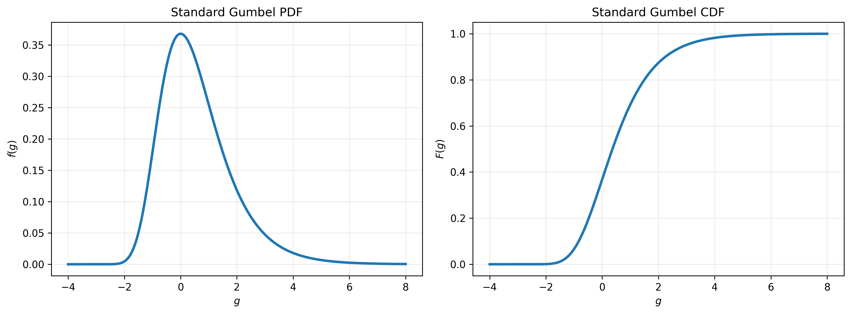
The Gumbel distribution originally arose in extreme value theory, where it models the distribution of maxima of random variables [2]. Surprisingly, this same distribution possesses a remarkable property that allows exact sampling from categorical distributions. The probability density function (PDF) of a standard Gumbel random variable is

[math]
f(g)=e^{-(g+e^{-g})},
\qquad g\in\mathbb{R},
[/math]

while its cumulative distribution function (CDF) is

[math]
F(g)=e^{-e^{-g}}.
[/math]

Two side-by-side plots depicting the Standard Gumbel Probability Density Function (PDF) on the left and the Cumulative Distribution Function (CDF) on the right. The PDF shows a pronounced peak around g = 0, while the CDF demonstrates a gradual increase approaching 1 as g increases.

Fortunately, generating Gumbel random variables is remarkably simple. Starting from a uniformly distributed random variable

[math]
u\sim\mathcal U(0,1),
[/math]

a standard Gumbel random variable is obtained through the transformation

[math]
g=-\log(-\log u).
[/math]

This simple inverse-transform sampling procedure is widely used in practice.

The Gumbel-Max Trick

Neural networks typically produce a vector of logits

[math]
\ell_1,\ldots,\ell_K,
[/math]

which define a categorical distribution through the softmax function

[math]
p_i=
\frac{\exp(\ell_i)}
{\sum_{j=1}^{K}\exp(\ell_j)}.
[/math]

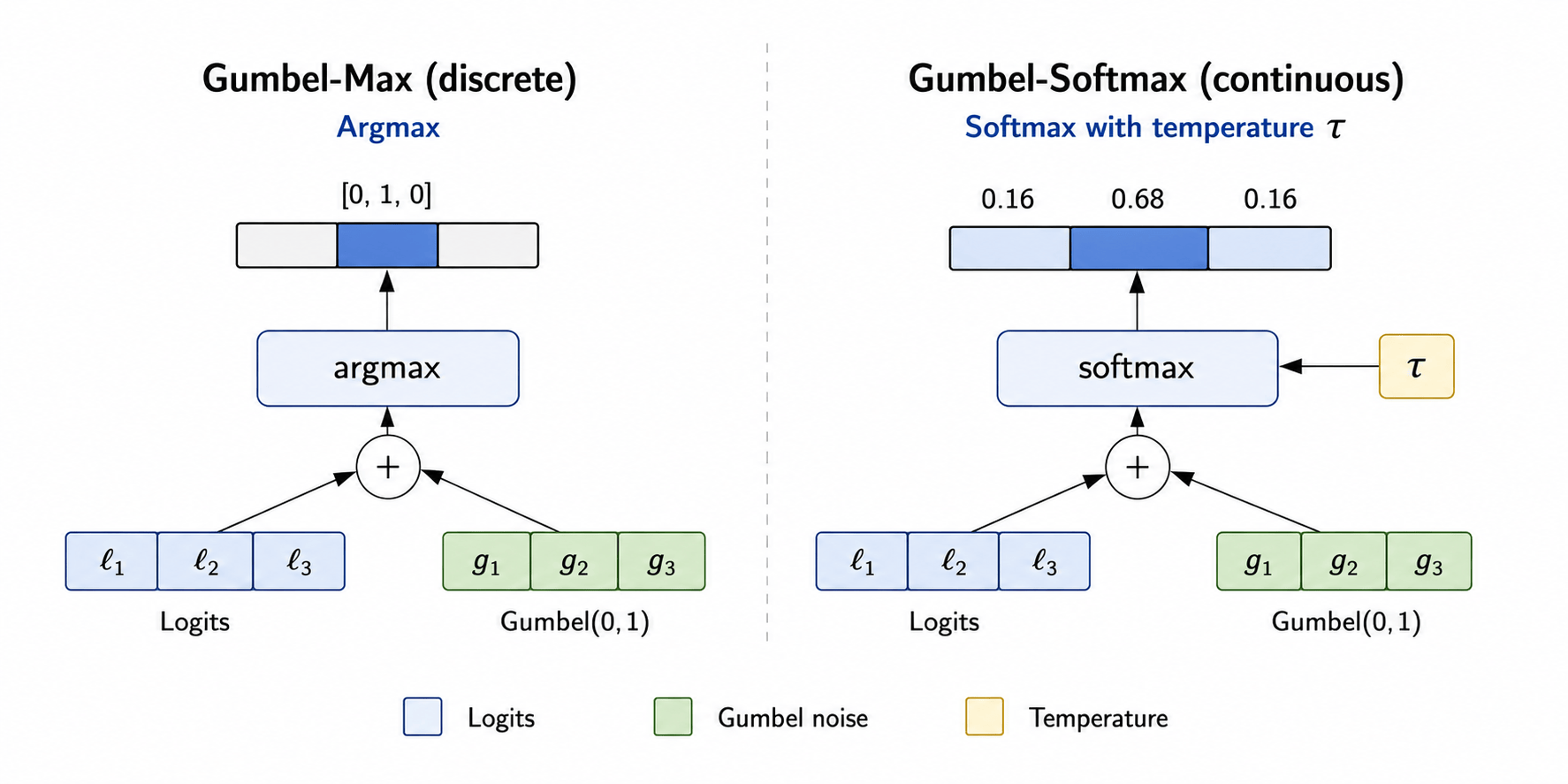
The Gumbel-Max trick provides an alternative way to sample from this distribution. It proceeds in three simple steps.

First, independently sample one standard Gumbel random variable for each possible outcome:

[math]
g_i\sim\mathrm{Gumbel}(0,1).
[/math]

Next, perturb each logit with its corresponding Gumbel noise:

[math]
s_i=\ell_i+g_i.
[/math]

Finally, select the outcome with the largest perturbed score:

[math]
m=\arg\max_i(\ell_i+g_i).
[/math]

At first sight, this procedure may seem surprising. Instead of directly sampling from the categorical probabilities, we add independent noise to every logit and then apply a deterministic argmax.

Yet the procedure is exact, not approximate. The selected index follows the original categorical distribution:

[math]
P(m=k)=p_k.
[/math]

Many presentations of the Gumbel-Max trick replace the logits [math]\ell_i[/math] with the log-probabilities [math]\log p_i[/math], leading to the equivalent expression

[math]
m=\arg\max_i(\log p_i+g_i).
[/math]

The two formulations are identical because [math]\log p_i[/math] differs from [math]\ell_i[/math] only by the additive constant [math]-\log\left(\sum_j e^{\ell_j}\right)[/math], which does not affect the outcome of the [math]\arg\max[/math]. In practice, deep learning implementations typically operate directly on the logits.

The intuition is that the logits determine the relative preference for each outcome, while the Gumbel variables introduce randomness into the competition between them. Outcomes with larger logits are more likely to win, but lower-probability outcomes can still be selected when they receive a sufficiently large noise value. The special form of the Gumbel distribution ensures that the resulting winning probabilities are exactly the softmax probabilities.

From Gumbel-Max to Gumbel-Softmax

Although the Gumbel-Max trick provides an elegant way to sample from a categorical distribution, it does not yet solve our original problem. The final operation is still

[math]
m=\arg\max_i(\ell_i+g_i),
[/math]

and the [math]\arg\max[/math] function is not differentiable.

The key idea behind Gumbel-Softmax is to replace only this final [math]\arg\max[/math] by a differentiable approximation [3], [4]. Instead of selecting the largest perturbed logit, we apply a softmax function to the perturbed logits:

[math]
y_i=
\frac{\exp((\ell_i+g_i)/\tau)}
{\sum_j\exp((\ell_j+g_j)/\tau)},
[/math]

where [math]\tau>0[/math] is the temperature parameter.

The output is now a continuous probability vector rather than a one-hot sample, making the entire computation differentiable and allowing gradients to propagate through standard backpropagation.

The temperature controls the quality of the approximation. High temperatures produce smooth probability vectors, whereas low temperatures yield increasingly sharp distributions that closely resemble the original Gumbel-Max samples.

Diagram comparing Gumbel-Max (discrete) and Gumbel-Softmax (continuous) methods, with argmax and softmax processes illustrated. Features logits, Gumbel noise, and temperature settings.

Main Properties

We now verify the main properties of the Gumbel-Softmax distribution through a series of simple experiments.

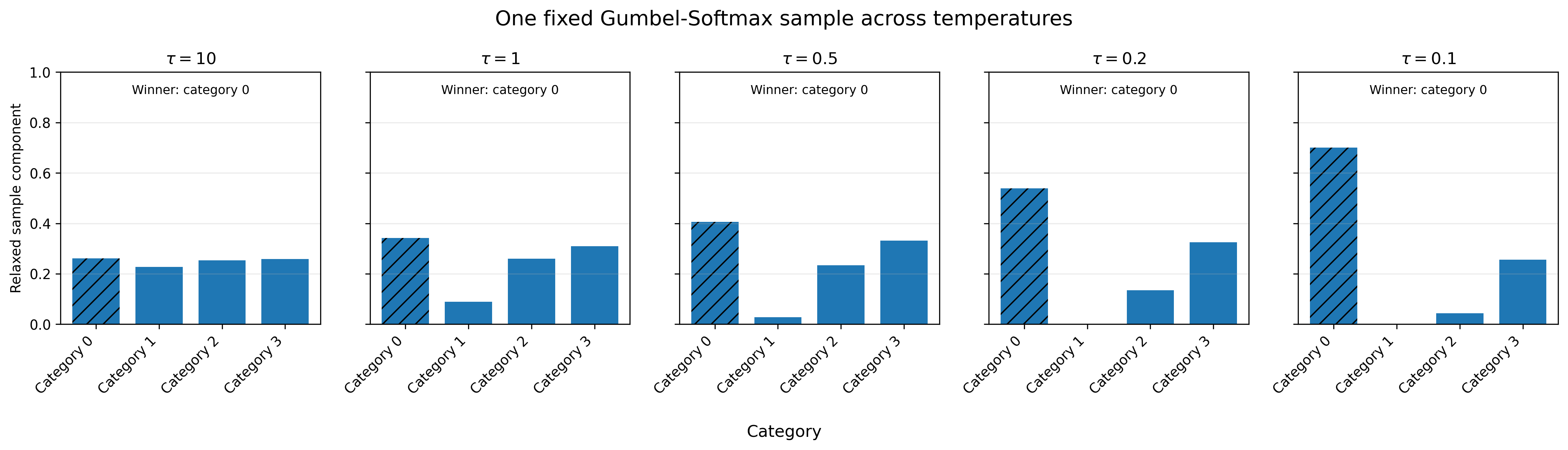
Property 1: Controlled Continuous Relaxation

We keep the same realization of Gumbel noise while varying only the temperature.

Bar charts showing the fixed Gumbel-Softmax sample across different temperatures (τ): 10, 1, 0.5, 0.2, and 0.1. Each chart displays the sample component for four categories, indicating the winning category for each temperature.

As the temperature decreases, the relaxed sample becomes increasingly concentrated on the same winning category. In the limit [math]\tau\rightarrow0[/math], the relaxed vector converges to the corresponding one-hot sample produced by the Gumbel-Max trick. Conversely, large temperatures produce smooth probability vectors that distribute their probability mass over several categories.

Property 2: Bias of the Relaxation

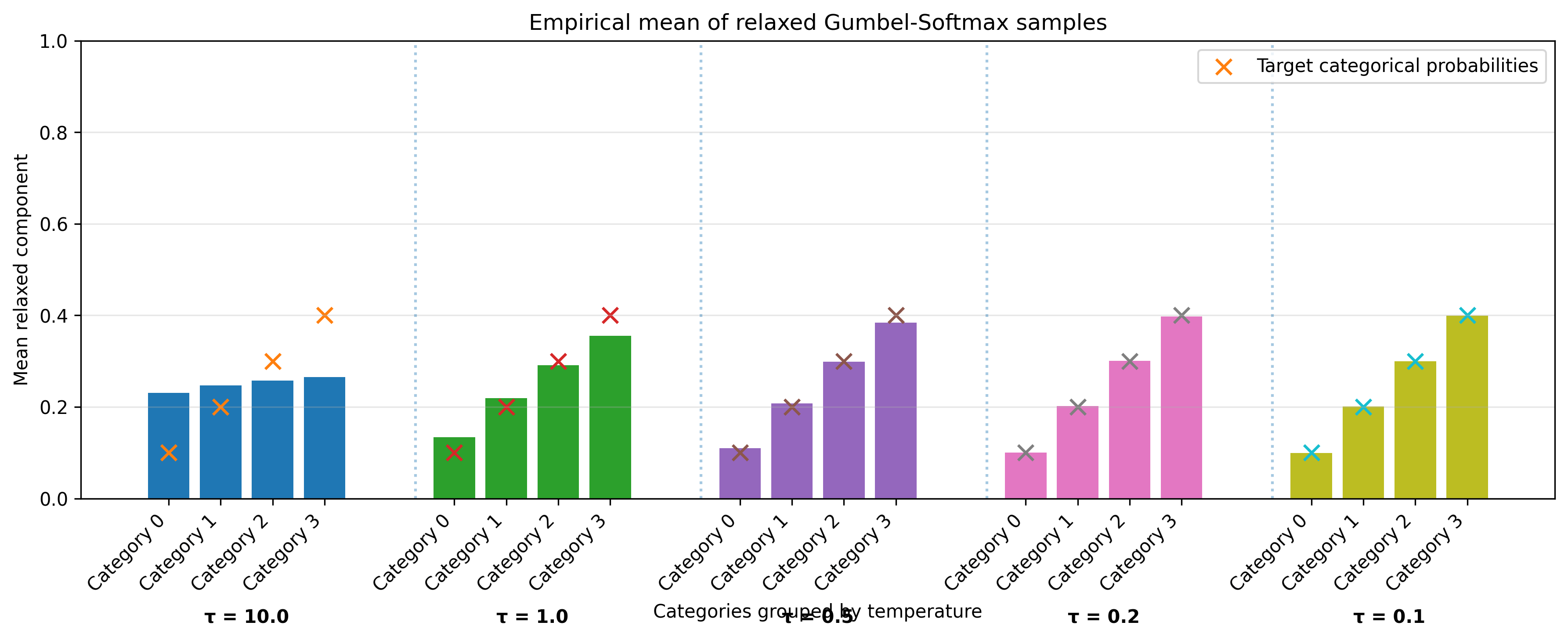
The Gumbel-Softmax output is a continuous probability vector rather than an exact one-hot categorical sample. Therefore, at a finite temperature, its expected value does not generally coincide with the target categorical distribution.

Bar chart showing the empirical mean of relaxed Gumbel-Softmax samples across different categories and temperatures (τ). Categories are labeled 0 to 3, with different colors representing varying temperatures (τ = 10.0, 1.0, 0.2, and 0.1). Target categorical probabilities are indicated by orange 'x' marks.

At high temperatures, the relaxed samples are strongly smoothed, and their empirical mean is pulled toward a more uniform distribution. As the temperature decreases, the samples become sharper and the empirical mean moves progressively closer to the target categorical probabilities. In the low-temperature regime, the relaxed distribution becomes nearly indistinguishable from the original categorical distribution.

Property 3: Exact Categorical Sampling

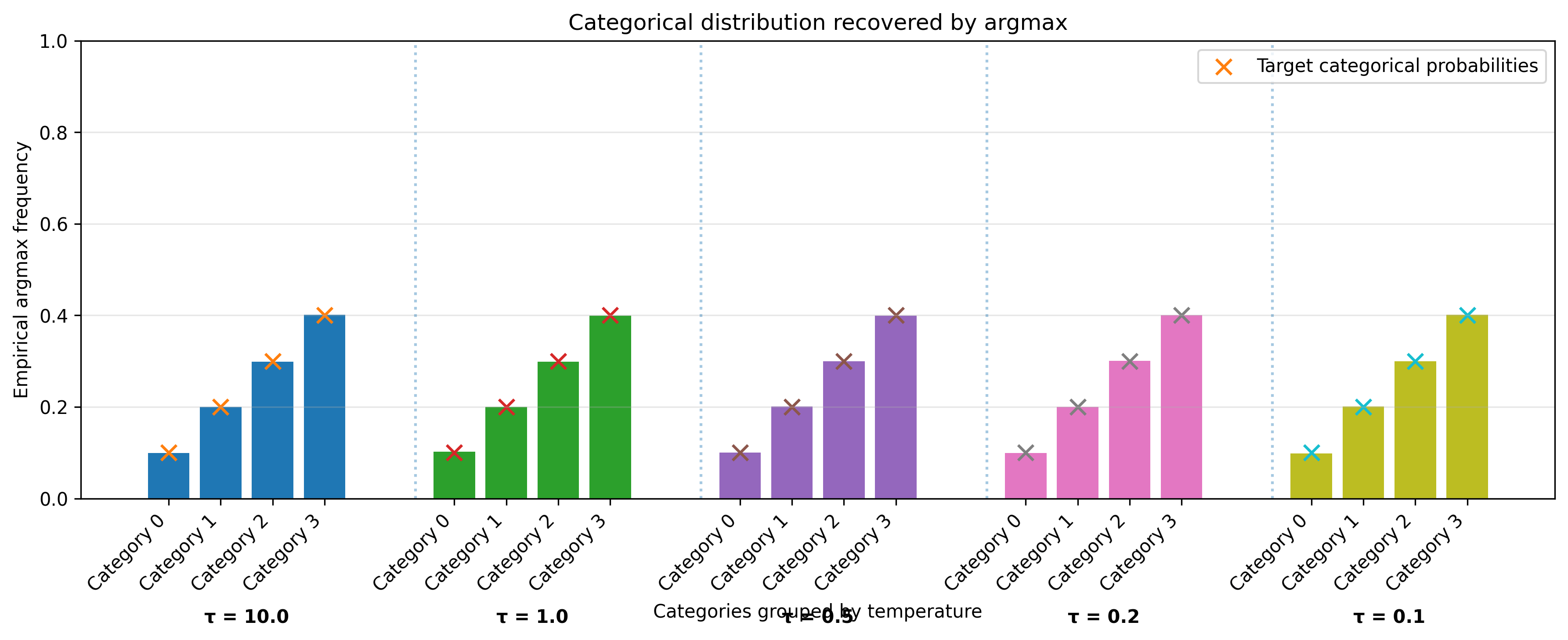
Although the relaxed samples are biased, the discrete samples obtained through the Gumbel-Max trick remain exact. Indeed, multiplying or dividing every perturbed logit by the same positive constant does not change their ordering. Therefore,

argmaxi(ℓi+giτ)=argmaxi(ℓi+gi),τ>0.\mathrm{argmax}_i\left(\frac{\ell_i+g_i}{\tau}\right) = \mathrm{argmax}_i\left(\ell_i+g_i\right), \qquad \tau>0.

Consequently, applying the [math]argmax[/math] to a Gumbel-Softmax sample always produces exactly the same discrete sample as the Gumbel-Max trick, regardless of the temperature.

Bar graph depicting the empirical argmax frequency of four categories across different temperature values (τ = 10.0, 1.0, 0.2, 0.1). Each category is represented with colored bars and target categorical probabilities marked with Xs.

Where is Gumbel-Softmax Useful?

The Gumbel-Softmax trick is useful whenever a neural network must make an internal discrete decision while still being trained end-to-end. Representative applications include experimental or differentiable formulations of:

  • Emergent languages – learning discrete communication symbols between agents, as demonstrated by Havrylov and Titov [5] and by Mordatch and Abbeel [6].
  • Discrete latent representations – variational autoencoders and other generative models.
  • Mixture-of-Experts routing – selecting which expert processes an input.
  • Memory and retrieval – selecting a memory slot or retrieved document.
  • Tool or module selection – routing inputs to specialized models or computational modules.

Conclusions

The Gumbel-Max trick provides an elegant way to sample exactly from a categorical distribution by adding Gumbel noise to the logits. Although the resulting sampling operation is not differentiable, it naturally leads to the Gumbel-Softmax relaxation.

By replacing the discrete one-hot sample with a continuous probability vector, the Gumbel-Softmax enables gradients to flow through discrete choices. The temperature parameter controls the trade-off between smooth differentiable samples and faithful approximations of the original categorical distribution.

Together, these two techniques have become fundamental tools for incorporating discrete random variables into end-to-end differentiable machine learning models.

I hope this blog has helped demystify this elegant idea.

References

[1] Diederik P. Kingma and Max Welling. Auto-Encoding Variational Bayes. International Conference on Learning Representations (ICLR), 2014.

[2] E. J. Gumbel, Statistics of Extremes, Columbia University Press, 1958.

[3] Eric Jang, Shixiang Gu, and Ben Poole. Categorical Reparameterization with Gumbel-Softmax. International Conference on Learning Representations (ICLR), 2017.

[4] Maddison, C. J., Mnih, A., & Teh, Y. W. (2017). The Concrete Distribution: A Continuous Relaxation of Discrete Random Variables. In Proceedings of the 5th International Conference on Learning Representations (ICLR 2017).

[5] Serhii Havrylov and Ivan Titov. Emergence of Language with Multi-Agent Games: Learning to Communicate with Sequences of Symbols. Advances in Neural Information Processing Systems (NeurIPS), 2017.

[6] Igor Mordatch and Pieter Abbeel. Emergence of Grounded Compositional Language in Multi-Agent Populations. AAAI Conference on Artificial Intelligence, 2018.

Cite as

@misc{giovanidis2026gumbel,
author = {Anastasios Giovanidis},
title = {Gumbel-softmax: Making Discrete Sampling Differentiable},
year = {2026},
howpublished = {\url{https://anastasiosgiovanidis.net/2026/07/20/gumbel-softmax-making-discrete-sampling-differentiable/}},
note = {Online tutorial}
}

Giovanidis, A. (2026). Gumbel-Softmax: Making Discrete Sampling Differentiable. anastasiosgiovanidis.net.

Leave a comment

Filed under Uncategorized

GRPO is just PPO for bandits

DeepSeek-R1 [1] is the first open-source model that exhibits comparable performance to closed source LLMs, by utilizing Reinforcement learning (RL) to improve reasoning ability after the Supervised Fine-Tuning (SFT) stage.

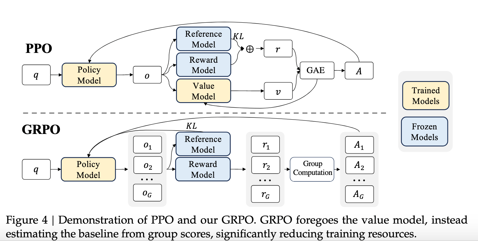
In a precursory LLM model named DeepSeekMath [2], the team introduced their RL method tagged Group Relative Policy Optimization (GRPO), which is a variant of Proximal Policy Optimization (PPO) [3].

Figure Source: DeepSeekMath [2]

This method is similar to PPO, and optimizes the memory usage by not relying on a learned value function approximation, which would be expensive in memory to maintain. It uses instead the average reward of multiple sampled outputs, produced in response to the same question, as the baseline. More specifically, for each question [math]q[/math], GRPO samples a group of outputs [math]\{o_1, o_2,\ldots, o_G\}[/math] from the old policy [math]\pi_{\theta_{old}}[/math], maps them to rewards [math]\{r_1, r_2,\ldots, r_G\}[/math] using a (possibly parameterized) reward function [math]r_i=r_{\phi}(o_i)[/math] and then optimizes the policy model by maximizing the following objective:

[math] \begin{align}J_{GRPO}(\theta) = \mathbb{E}_{[q\sim P(Q), \{o_i\}_{i=1}^G\sim \pi_{\theta_{old}}(O|q)]} \frac{1}{G}\sum_{i=1}^G \{f(\rho_{\theta},\hat{A}_i)-\beta D_{KL}[\pi_{\theta}||\pi_{ref}]\}\end{align}[/math]

The above objective is in expectation over the distribution of questions [math]P(Q)[/math] and the old policy [math]\pi_{\theta_{old}}[/math]. The function [math]f[/math] is the clipping formula using advantages [math]\hat{A}_i[/math]

[math]f(\rho_{\theta},\hat{A}_i) = \min\left[\rho_{\theta}\hat{A}_{i},clip(\rho_{\theta},1-\epsilon,1+\epsilon)\hat{A}_{i}\right][/math].

In the above expression, the policy ratios are defined as

[math]\begin{align}\rho_{\theta} = \frac{\pi_{\theta}(o_{i}|q)}{\pi_{\theta_{old}}(o_{i}|q)}\end{align}[/math],

and the advantage is defined using only the rewards from collected observations

[math]\begin{align} \hat{A}_i=\frac{r_i-mean(r_1,\ldots,r_G)}{std(r_1,\ldots,r_G)}\end{align}[/math].

Furthermore, the Kullback-Leibler (KL) divergence in the expression aims to keep the policy [math]\pi_{\theta}[/math] as close as possible to the SFT initial phase [math]\pi_{ref}[/math]. It actually uses an unbiased estimator [4] from each sample of question-answer [math](q,o_i)[/math]

[math]\begin{align}D_{KL}[\pi_{\theta}||\pi_{ref}]\} \approx \frac{\pi_{ref}(o_i|q)}{\pi_{\theta}(o_i|q)}- \log\frac{\pi_{ref}(o_i|q)}{\pi_{\theta}(o_i|q)} – 1\end{align}[/math].

An intuitive presentation of GRPO is presented in [5].

Here we present a simple way to derive the GRPO step by step using its building blocks. Essentially we will show that GRPO is a policy gradient method for immediate rewards, similar to bandit algorithms.

Step 1: Policy gradient for one-step rewards

The GRPO as so many other RL algorithms aims to find a policy [math]\pi_{\theta^*}[/math] to maximize the expected reward. The randomness is from the environment, i.e. the person asking the question, as well as the learned policy which can be probabilistic. Here, someone is asking a question [math]q[/math] following some distribution [math]P(q)[/math]. The objective to be maximized is

[math]\begin{align}J(\theta) = \mathbb{E}_{\pi_{\theta}}[r_{t_0}+\gamma r_{t_1}+\gamma^2 r_{t_2}+\ldots] \stackrel{\gamma=0}{\rightarrow}\mathbb{E}_{\pi_{\theta}}[r_{t_0}]= \sum_{q\in Q}d(q)\sum_{o\in O}\pi_{\theta}(o|q)r(o,q) \end{align}[/math],

where [math]d(q)[/math] is the frequency of requesting question [math]q[/math]. In the single hop (bandit) case, where the discount factor is zero, one can realize that there is no need to refer to the Policy Gradient Theorem [9] because the only dependence on [math]\theta[/math] is on the policy and not on some value function because only the immediate reward counts. Then we write

[math]\begin{align}\nabla_{\theta}J(\theta) = \sum_{q\in Q}d(q)\sum_{o\in O}r(o,q)\nabla_{\theta}\pi_{\theta}(o|q) = \mathbb{E}_{q\sim P(q), o\sim \pi_{\theta}}\left[r(o,q)\nabla_{\theta}\log(\pi_{\theta}(o|q))\right]\end{align}[/math].

Note that we can use the empirical average to approximate the expectation over the policy output. As GRPO claims, we sample [math]\{o_1,\ldots,o_G\}[/math] answers for the question q, using our current formula, and approximate the above gradient by the empirical one

[math]\begin{align}\nabla_{\theta}J(\theta) \approx \mathbb{E}_{q\sim P(q), \{o_1,\ldots,o_G\}\sim \pi_{\theta}}\frac{1}{G}\sum_{i=1}^G\left(r(o_i,q)\nabla_{\theta}\log(\pi_{\theta}(o_i|q))\right)\end{align}[/math].

Step 2: Generalized Advantage

In the above, the immediate reward [math]r(o,q)[/math] takes the place of the state-action value function [math]Q_{\theta}(o,q)[/math] of the standard policy gradient. From [6], it is very usual to replace in the policy gradient the state-action value function by the advantage [math]A(o,q)= Q_{\theta}(o,q)-V(s)[/math]. In practice [7], instead of subtracting from each [math]Q_{\theta}(o,q)[/math] the maximum value function among all possible answers [math]\max_o Q_{\theta}(o,q)[/math] we can also subtract the average over all possible actions from the set [math]O[/math]

[math]\begin{align}A(o,q)= Q_{\theta}(o,q)-\frac{1}{|O|}\sum_{i=1}^O Q_{\theta}(o_i,q)\stackrel{\gamma=0}{\rightarrow} A(o,q)= r(o,q)-\frac{1}{|O|}\sum_{i=1}^O r(o_i,q)\end{align}[/math].

Since we cannot have the entire range of answers available, we use here in the GRPO the available answers [math]\{o_1,\ldots,o_G\}[/math] only. Combining the above two steps we would like to maximize the following objective

[math]\begin{align}\max_{\theta} \ L^{Policy Gradient}(\theta) = \mathbb{E}_{q\sim P(q), o\sim\pi_{\theta}}\left[A(o,q)\log(\pi_{\theta}(o|q))\right]\end{align}[/math].

Step 3: TRPO

In the TRPO paper [8] the above objective is replaced by a surrogate objective

[math]\begin{align}\max_{\theta} \ L^{TRPO}(\theta) = \mathbb{E}_{q\sim P(q), o\sim\pi_{\theta_{old}}}\left[A_{old}(o,q)\frac{\pi_{\theta}(o|q)}{\pi_{\theta_{old}}(o|q)})\right]\end{align}[/math].

We consider the policy is updated step-wise. Once we have some version [math]\pi_{\theta_{old}}(o|q)[/math] we collect observations [math]\{o_1,\ldots,o_G\}[/math], calculate the advantages and plug this information in the above formula to update the policy. From an intuitive point of view, [math]L^{TRPO}(\theta)[/math] and [math]L^{Policy Gradient}(\theta)[/math] are very similar to each other. Remember that the derivative of the latter is

[math]\begin{align}\mathbb{E}[A(o,q)\nabla\log{\pi_{\theta}(o|q)}] = \mathbb{E}\left[A(o,q)\frac{\nabla\pi_{\theta}(o|q)}{\pi_{\theta}(o|q)}\right]\stackrel{freeze\theta_{old}}{=} \mathbb{E}\left[A_{old}(o,q)\frac{\nabla\pi_{\theta}(o|q)}{\pi_{\theta_{old}}(o|q)}\right] \end{align}[/math]

Then, obviously the right-hand side is just the derivative of [math]L^{TRPO}(\theta)[/math].

Step 4: PPO

The PPO paper introduces the clipped surrogate objective function [math]f(\rho_{\theta},\hat{A}_i) = \min\left[\rho_{\theta}\hat{A}_{i},clip(\rho_{\theta},1-\epsilon,1+\epsilon)\hat{A}_{i}\right][/math] that we saw above in the GRPO, in order to bound the steps of the new policy update compared to the old policy. The aim is to keep the next update close to the previous one. If the advantage is positive and the new policy favors this compared to the old policy then the function clips above to [math]1+\epsilon[/math] how much the improvement can allowed to be. In the case of negative advantage, if the new policy defavorizes it, then the reduction is clipped below by [math]1-\epsilon[/math].

Finally, the Kullback-Leibler divergence of the new policy compared to the reference one, further limits the update step to keep it close to SFT which has been trained on acceptable and desirable outcomes.

Conclusion

It is important to observe that the PPO value function estimation was never necessary in the first place. The question-answer problem is one-hop and hence similar to the bandit problems. This was already mentioned in the paper [10]: “The environment is a bandit environment which presents a random customer prompt and expects a response to the prompt. Given the prompt and response, it produces a reward determined by the reward model and ends the episode.”

Consequently, the importance in the GRPO lies in the relation between the reward mapping [math]r_{\phi}(o)[/math], the policy-gradient, and how many samples G can be collected (which in LLMs is expensive). Also, rather important seems to be the answer sampling policy. Such a discussion and the sensitivity of the outcome with respect to the design of the reward function has been shown in the very nice analysis by Marc Lelarge in his GitHub page [11].

Realizing that GRPO is just a sophisticated bandit algorithm, maybe other methods in the future can establish as good or better convergence. On the other hand, there could be interest to study how a sequence of questions-answers can be trained using classic PPO, maybe producing more interesting tuning since it will account for chain of interactions, instead of single-hop.

@article{giovanidis2025_GRPO,
title = “GRPO is just PPO for Bandits”,
author = “Giovanidis, Anastasios”,
journal = “anastasiosgiovanidis.net”,
year = “2025”,
url = “https://anastasiosgiovanidis.net/2025/02/17/grpo-is-just-ppo-for-bandits/“
}

References

[1] DeepSeek-AI “DeepSeek-R1: Incentivizing Reasoning Capability in LLMs via Reinforcement Learning”, arXiv:2501.12948

[2] Shao et al. “DeepSeekMath: Pushing the Limits of Mathematical Reasoning in Open Language Models”, arXiv:2402.03300v3

[3] Proximal Policy Optimization Algorithms, Schulman et al. 2017, arXiv:1707.06347v2

[4] John Schulmans’ homepage “Approximating KL Divergence” http://joschu.net/blog/kl-approx.html

[5] https://iaee.substack.com/p/deepseek-r1-intuitively-and-exhaustively

[6] Schulman et al “High-Dimensional Continuous Control Using Generalized Advantage Estimation” arXiv:1506.02438v6

[7] Wang et al “Dueling Network Architectures for Deep Reinforcement Learning”, arXiv:1511.06581v3

[8] Schulman et al “Trust Region Policy Optimization”, arXiv:1502.05477

[9] Sutton et al. “Policy Gradient Methods for Reinforcement Learning with Function Approximation“, NeurIPS 1999

[10] Ouyang et al. “Training language models to follow instructions with human feedback”, arXiv:2203.02155v1

[11] https://github.com/dataflowr/notebooks/blob/master/llm/Gauss_GRPO.ipynb

Leave a comment

Filed under Uncategorized

WIOPT 2017 CfP

==========================================================================

WiOpt 2017, The 15th International Symposium on Modeling and Optimization in Mobile, Ad Hoc, and Wireless Networks (http://wiopt.telecom-paristech.fr)

Telecom ParisTech, Paris, France, May 15-19th, 2017

==========================================================================

Important Dates

Paper registration: December 15, 2016
Paper submission: December 22, 2016
Notification of acceptance: February 17, 2017
Camera ready and Registration: March 17, 2017
Conference: May 15-19, 2017

WiOpt 2017 is technically co-sponsored by the IEEE Control Systems Society, IEEE Information Theory Society and IFIP. All papers will be published in the IFIP DL open library with Open Access, as well as on IEEE Xplore.

==========================================================================

The 15th International Symposium on Modeling and Optimization in Mobile, Ad Hoc, and Wireless Networks solicits high-quality contributions.

WiOpt 2017 welcomes original papers related to modeling, performance evaluation, and optimization of wireless networks. The scope covers all types of wireless networks: cellular, ad hoc, content-driven, delay-tolerant, mesh, metropolitan, sensor, cognitive, vehicular, robotic, Internet of Things, virtualized, etc. The focus is on issues at and above the MAC layer, although cross-layer techniques encompassing the physical layer are equally welcome. We encourage both theoretical contributions and submissions relating to real world empirical measurements, experimental studies. The areas of interest include, but are not limited to:

– Modeling, model validation, and performance analysis
– Scaling laws and fundamental limits
– Network architectures
– Protocol design
– Resource allocation and management
– Packet scheduling
– Access control
– Network economics
– Quality of service
– Energy efficiency, harvesting, power control and management
– Security, trust and privacy
– Network resilience, anomaly detection, and reliability analysis
– Cross-layer design and optimization / control
– Measurements and experimental studies
– Data collection and storage
– Data analytics for wireless networks

==========================================================================

Committees

General Chairs: Marceau Coupechoux (Telecom ParisTech), Anastasios Giovanidis (CNRS, Telecom ParisTech), Jean Walrand (UC Berkeley)

TPC Chairs: Thomas Bonald (Telecom ParisTech), Mérouane Debbah (CentraleSupélec, HUAWEI), Jianwei Huang (CUHK), Muriel Médard (MIT)

Steering Committee

Eitan Altman (INRIA, France)
Tamer Basar (University of Illinois at Urbana–Champaign, USA)
Mung Chiang (Princeton University, USA)
Jon Crowcroft (University of Cambridge, UK)
Song Chong (Korea Advanced Institute of Science and Technology [KAIST], South Korea)
Marco Conti (Istituto di Informatica e Telematica, Italy)
Anthony Ephremides (University of Maryland, USA)
Krishna Jagannathan (Indian Institute of Technology [IIT] Madras, India)
Jie Li (University of Tsukuba, Japan)
Ariel Orda (Technion, Israel)
Gaurav Raina (Indian Institute of Technology [IIT] Madras, India)
Stavros Toumpis (Athens University of Economics and Business, Greece)

Leave a comment

Filed under Uncategorized

WIOPT 2017 in Paris, France!

We are organising the 15th edition of the International Symposium on Modeling and Optimization in Mobile, Ad Hoc, and Wireless Networks (WIOPT) in Paris France, together with Marceau Coupechoux (Telecom ParisTech) and Jean Walrand (UC Berkeley). The conference will take place in the grounds of the Telecom ParisTech school, between 15-19 May 2017, right in the heart of Paris.

Here is a link to our new WIOPT’17 web-site!

As part of the general conference, four additional workshops will accompany the main event:

– RAWNET, SpaSWiN, CCDWN, and GREENNET.

Don’t miss it!

Leave a comment

Filed under Uncategorized