
Published: July 2026 • Reading time: 15 min
Modern language models assign probabilities to every possible next token, but ultimately they must choose just one. This illustrates a fundamental challenge in machine learning: language and many other decision processes are inherently discrete, while neural networks are trained through continuous optimization. More generally, how can we sample discrete values while still training differentiable models?
One possibility is to treat sampling as a black-box stochastic operation and rely on reinforcement learning techniques such as REINFORCE to estimate gradients.
Another, remarkably elegant solution, is to reformulate the sampling process itself: Rather than viewing sampling as an opaque random operation, we express it as a deterministic function of the model parameters and an independent source of random noise. This seemingly small change opens the door to differentiable approximations that can be optimized efficiently using standard backpropagation.
This post explores one of the most influential ideas in this direction: the Gumbel-Max trick and its differentiable relaxation, the Gumbel-Softmax distribution.
Open the Gumbel-Softmax notebook in Google Colab
The Categorical Distribution
The mathematical object behind next-token prediction is the categorical distribution. Given a vocabulary of [math]K[/math] possible tokens, a neural network predicts a probability vector
[math]
\mathbf{p}=(p_1,p_2,\ldots,p_K),
[/math]
where
[math]
\sum_{i=1}^{K} p_i = 1,
\qquad
p_i \ge 0.
[/math]
Each probability represents how likely the corresponding token is to be selected. During inference, one token is sampled according to this distribution.
For example, suppose a language model predicts the following probabilities for the next word:
| Token | Probability |
|---|---|
| cat | 0.50 |
| dog | 0.30 |
| bird | 0.15 |
| fish | 0.05 |
The model will generate cat about half of the time, dog roughly one third of the time, and so on.
Training the neural network is straightforward because the probabilities depend smoothly on the model parameters. The difficulty appears only when we actually sample a token. Once a single token has been selected, the sampling process becomes discrete, and gradients can no longer naturally propagate through it.
This naturally raises the following question: can we sample from a categorical distribution in a different way, so that the sampled outcome becomes a deterministic function of the model parameters and an independent source of randomness? If so, the sampling operation itself becomes differentiable, allowing gradients to propagate through it during backpropagation.
The Reparameterization Trick
For continuous random variables, this idea is already well established through the reparameterization trick. Consider a Gaussian random variable
[math]
x\sim\mathcal N(\mu,\sigma^2).
[/math]
Rather than sampling [math]x[/math] directly, we first generate
[math]
\epsilon\sim\mathcal N(0,1),
[/math]
and then compute
[math]
x=\mu+\sigma\epsilon.
[/math]
The randomness is now entirely contained in the parameter-free variable [math]\epsilon[/math]. Once [math]\epsilon[/math] has been sampled, [math]x(\mu,\sigma;\epsilon)=\mu+\sigma\epsilon[/math] is a deterministic and differentiable function of [math]\mu[/math] and [math]\sigma[/math]. This simple reformulation enables gradients to propagate through the sampling process and forms the basis of Variational Autoencoders (VAEs) [1].

Can we construct an analogous reparameterization for discrete random variables? The answer is yes, and it begins with an unexpected distribution: the Gumbel distribution.
The Gumbel Distribution
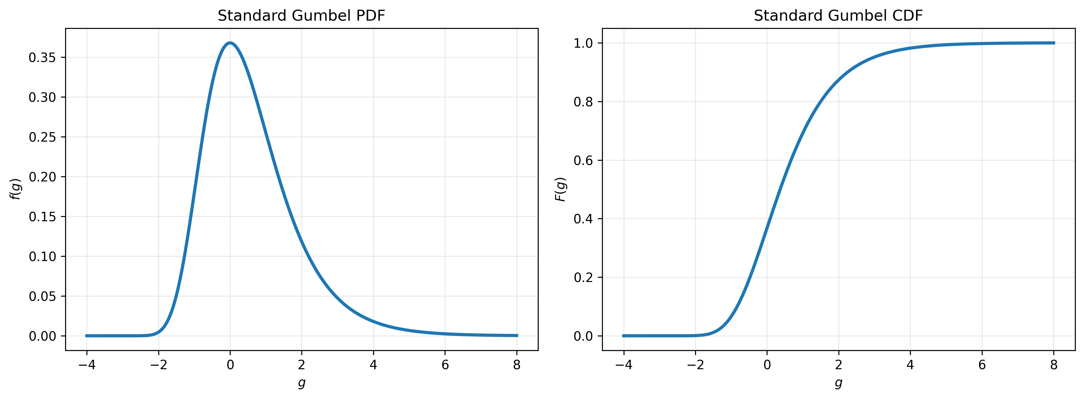
The Gumbel distribution originally arose in extreme value theory, where it models the distribution of maxima of random variables [2]. Surprisingly, this same distribution possesses a remarkable property that allows exact sampling from categorical distributions. The probability density function (PDF) of a standard Gumbel random variable is
[math]
f(g)=e^{-(g+e^{-g})},
\qquad g\in\mathbb{R},
[/math]
while its cumulative distribution function (CDF) is
[math]
F(g)=e^{-e^{-g}}.
[/math]
Fortunately, generating Gumbel random variables is remarkably simple. Starting from a uniformly distributed random variable
[math]
u\sim\mathcal U(0,1),
[/math]
a standard Gumbel random variable is obtained through the transformation
[math]
g=-\log(-\log u).
[/math]
This simple inverse-transform sampling procedure is widely used in practice.
The Gumbel-Max Trick
Neural networks typically produce a vector of logits
[math]
\ell_1,\ldots,\ell_K,
[/math]
which define a categorical distribution through the softmax function
[math]
p_i=
\frac{\exp(\ell_i)}
{\sum_{j=1}^{K}\exp(\ell_j)}.
[/math]
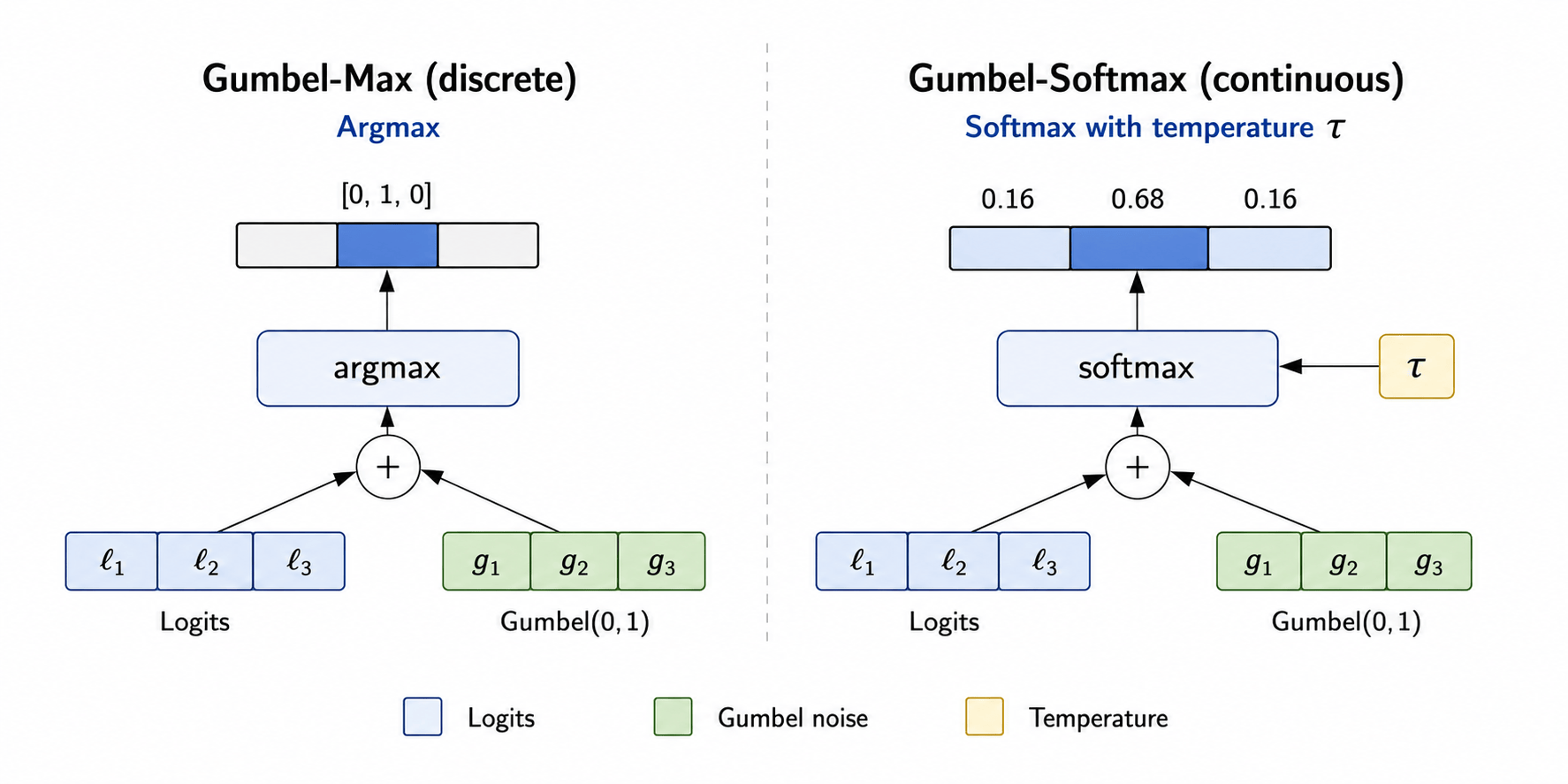
The Gumbel-Max trick provides an alternative way to sample from this distribution. It proceeds in three simple steps.
First, independently sample one standard Gumbel random variable for each possible outcome:
[math]
g_i\sim\mathrm{Gumbel}(0,1).
[/math]
Next, perturb each logit with its corresponding Gumbel noise:
[math]
s_i=\ell_i+g_i.
[/math]
Finally, select the outcome with the largest perturbed score:
[math]
m=\arg\max_i(\ell_i+g_i).
[/math]
At first sight, this procedure may seem surprising. Instead of directly sampling from the categorical probabilities, we add independent noise to every logit and then apply a deterministic argmax.
Yet the procedure is exact, not approximate. The selected index follows the original categorical distribution:
[math]
P(m=k)=p_k.
[/math]
Many presentations of the Gumbel-Max trick replace the logits [math]\ell_i[/math] with the log-probabilities [math]\log p_i[/math], leading to the equivalent expression
[math]
m=\arg\max_i(\log p_i+g_i).
[/math]
The two formulations are identical because [math]\log p_i[/math] differs from [math]\ell_i[/math] only by the additive constant [math]-\log\left(\sum_j e^{\ell_j}\right)[/math], which does not affect the outcome of the [math]\arg\max[/math]. In practice, deep learning implementations typically operate directly on the logits.
The intuition is that the logits determine the relative preference for each outcome, while the Gumbel variables introduce randomness into the competition between them. Outcomes with larger logits are more likely to win, but lower-probability outcomes can still be selected when they receive a sufficiently large noise value. The special form of the Gumbel distribution ensures that the resulting winning probabilities are exactly the softmax probabilities.
From Gumbel-Max to Gumbel-Softmax
Although the Gumbel-Max trick provides an elegant way to sample from a categorical distribution, it does not yet solve our original problem. The final operation is still
[math]
m=\arg\max_i(\ell_i+g_i),
[/math]
and the [math]\arg\max[/math] function is not differentiable.
The key idea behind Gumbel-Softmax is to replace only this final [math]\arg\max[/math] by a differentiable approximation [3], [4]. Instead of selecting the largest perturbed logit, we apply a softmax function to the perturbed logits:
[math]
y_i=
\frac{\exp((\ell_i+g_i)/\tau)}
{\sum_j\exp((\ell_j+g_j)/\tau)},
[/math]
where [math]\tau>0[/math] is the temperature parameter.
The output is now a continuous probability vector rather than a one-hot sample, making the entire computation differentiable and allowing gradients to propagate through standard backpropagation.
The temperature controls the quality of the approximation. High temperatures produce smooth probability vectors, whereas low temperatures yield increasingly sharp distributions that closely resemble the original Gumbel-Max samples.
Main Properties
We now verify the main properties of the Gumbel-Softmax distribution through a series of simple experiments.
Property 1: Controlled Continuous Relaxation
We keep the same realization of Gumbel noise while varying only the temperature.
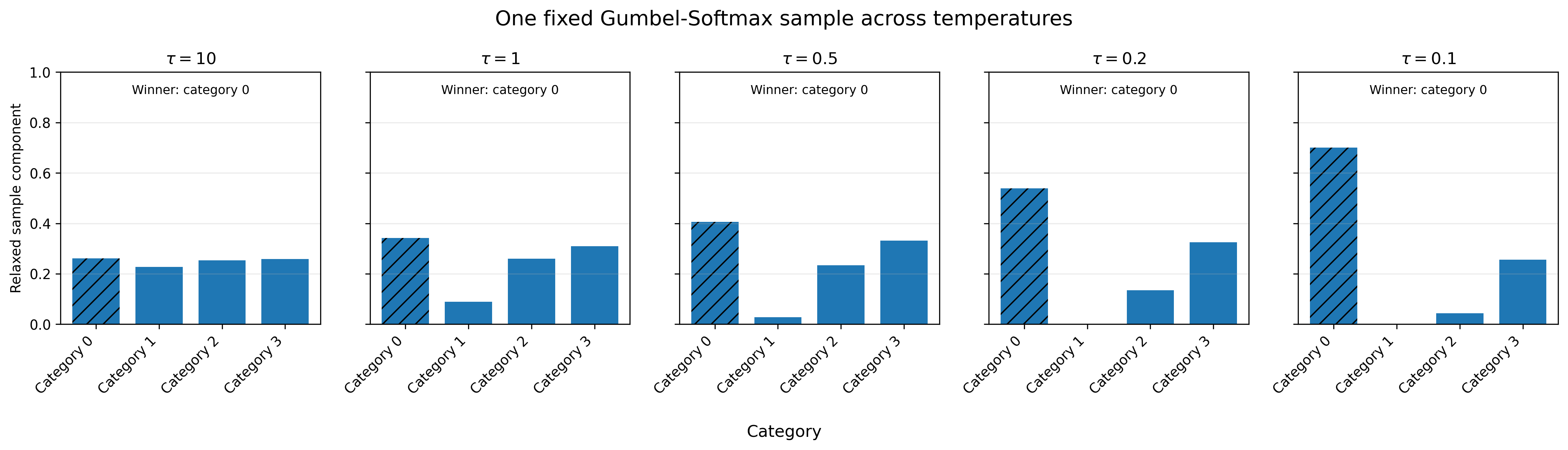
As the temperature decreases, the relaxed sample becomes increasingly concentrated on the same winning category. In the limit [math]\tau\rightarrow0[/math], the relaxed vector converges to the corresponding one-hot sample produced by the Gumbel-Max trick. Conversely, large temperatures produce smooth probability vectors that distribute their probability mass over several categories.
Property 2: Bias of the Relaxation
The Gumbel-Softmax output is a continuous probability vector rather than an exact one-hot categorical sample. Therefore, at a finite temperature, its expected value does not generally coincide with the target categorical distribution.
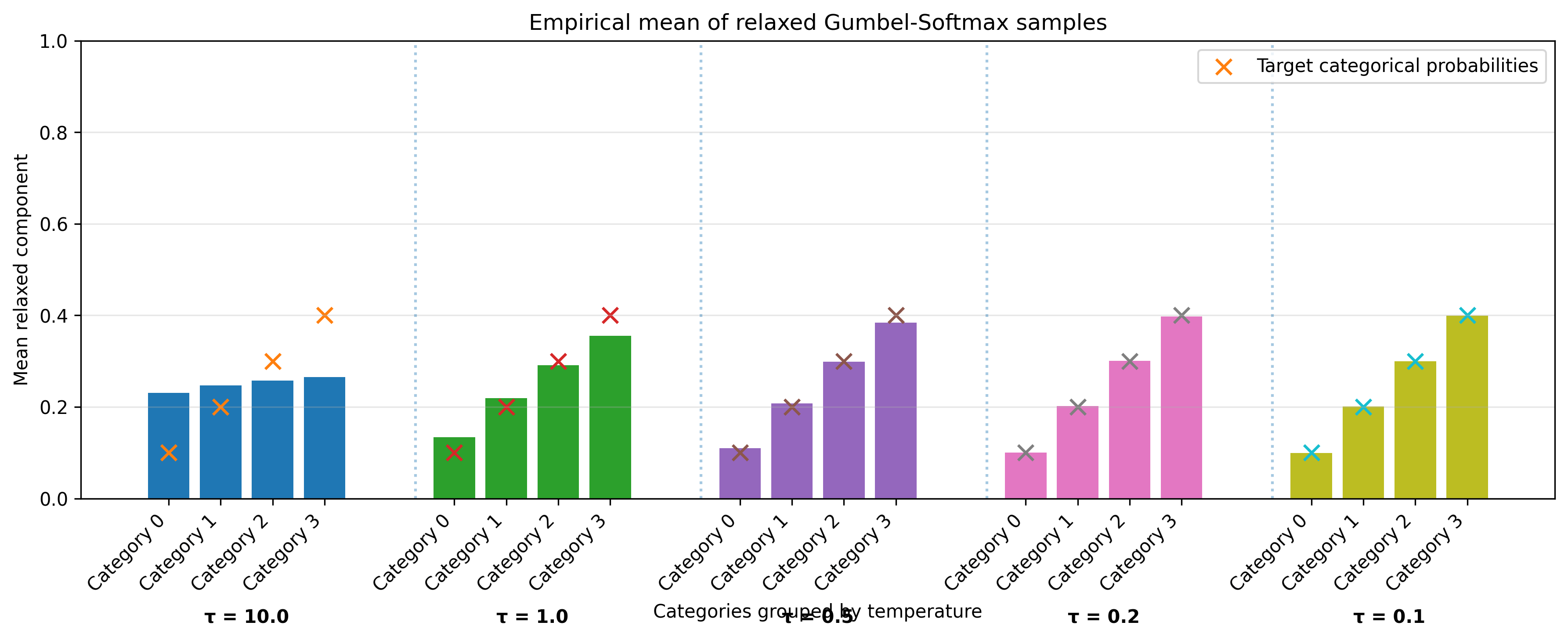
At high temperatures, the relaxed samples are strongly smoothed, and their empirical mean is pulled toward a more uniform distribution. As the temperature decreases, the samples become sharper and the empirical mean moves progressively closer to the target categorical probabilities. In the low-temperature regime, the relaxed distribution becomes nearly indistinguishable from the original categorical distribution.
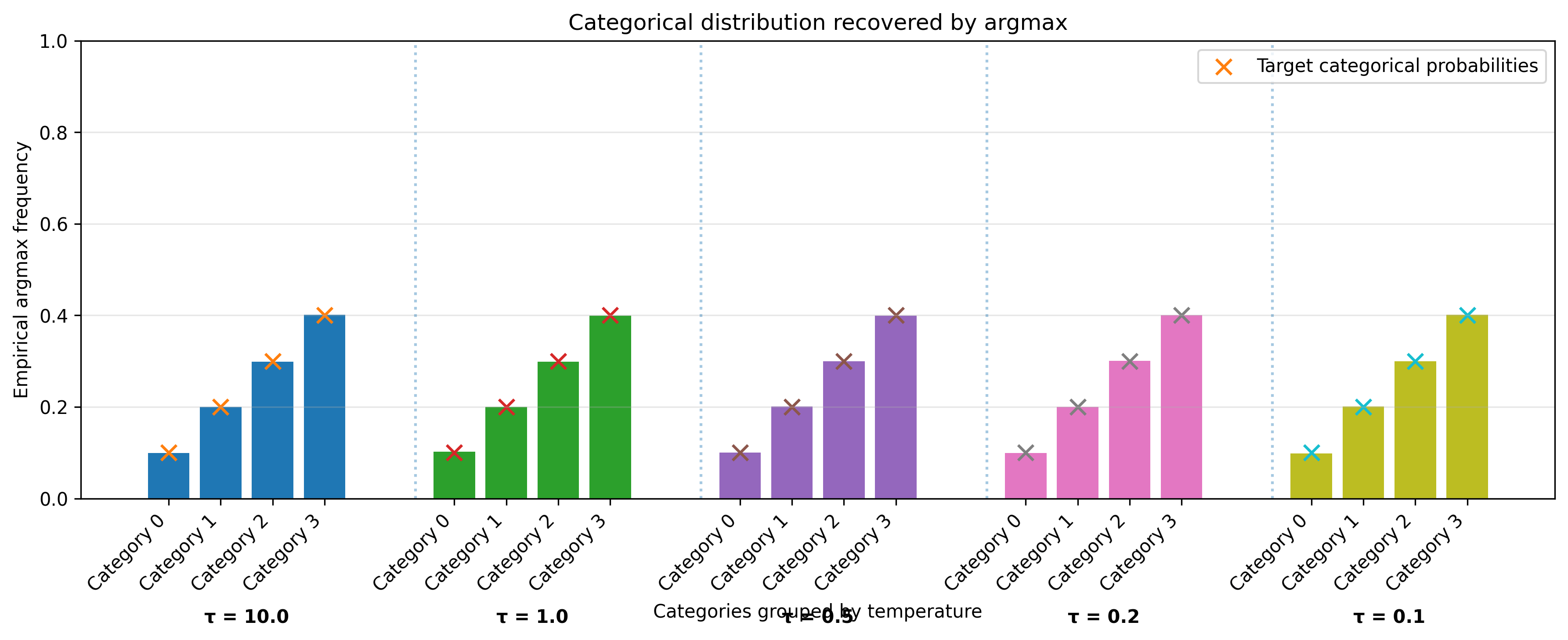
Property 3: Exact Categorical Sampling
Although the relaxed samples are biased, the discrete samples obtained through the Gumbel-Max trick remain exact. Indeed, multiplying or dividing every perturbed logit by the same positive constant does not change their ordering. Therefore,
Consequently, applying the [math]argmax[/math] to a Gumbel-Softmax sample always produces exactly the same discrete sample as the Gumbel-Max trick, regardless of the temperature.
Where is Gumbel-Softmax Useful?
The Gumbel-Softmax trick is useful whenever a neural network must make an internal discrete decision while still being trained end-to-end. Representative applications include experimental or differentiable formulations of:
- Emergent languages – learning discrete communication symbols between agents, as demonstrated by Havrylov and Titov [5] and by Mordatch and Abbeel [6].
- Discrete latent representations – variational autoencoders and other generative models.
- Mixture-of-Experts routing – selecting which expert processes an input.
- Memory and retrieval – selecting a memory slot or retrieved document.
- Tool or module selection – routing inputs to specialized models or computational modules.
Conclusions
The Gumbel-Max trick provides an elegant way to sample exactly from a categorical distribution by adding Gumbel noise to the logits. Although the resulting sampling operation is not differentiable, it naturally leads to the Gumbel-Softmax relaxation.
By replacing the discrete one-hot sample with a continuous probability vector, the Gumbel-Softmax enables gradients to flow through discrete choices. The temperature parameter controls the trade-off between smooth differentiable samples and faithful approximations of the original categorical distribution.
Together, these two techniques have become fundamental tools for incorporating discrete random variables into end-to-end differentiable machine learning models.
I hope this blog has helped demystify this elegant idea.
References
[1] Diederik P. Kingma and Max Welling. Auto-Encoding Variational Bayes. International Conference on Learning Representations (ICLR), 2014.
[2] E. J. Gumbel, Statistics of Extremes, Columbia University Press, 1958.
[3] Eric Jang, Shixiang Gu, and Ben Poole. Categorical Reparameterization with Gumbel-Softmax. International Conference on Learning Representations (ICLR), 2017.
[4] Maddison, C. J., Mnih, A., & Teh, Y. W. (2017). The Concrete Distribution: A Continuous Relaxation of Discrete Random Variables. In Proceedings of the 5th International Conference on Learning Representations (ICLR 2017).
[5] Serhii Havrylov and Ivan Titov. Emergence of Language with Multi-Agent Games: Learning to Communicate with Sequences of Symbols. Advances in Neural Information Processing Systems (NeurIPS), 2017.
[6] Igor Mordatch and Pieter Abbeel. Emergence of Grounded Compositional Language in Multi-Agent Populations. AAAI Conference on Artificial Intelligence, 2018.
Cite as
@misc{giovanidis2026gumbel,
author = {Anastasios Giovanidis},
title = {Gumbel-softmax: Making Discrete Sampling Differentiable},
year = {2026},
howpublished = {\url{https://anastasiosgiovanidis.net/2026/07/20/gumbel-softmax-making-discrete-sampling-differentiable/}},
note = {Online tutorial}
}
Giovanidis, A. (2026). Gumbel-Softmax: Making Discrete Sampling Differentiable. anastasiosgiovanidis.net.