
This blog-post treats the quantile and expectile regression for linear and non-linear regression. It highlights its differences with standard loss functions such as MSE, and showcases the extra information that the approach provides. Applications of this type of regression to Reinforcement Learning (Temporal Difference) is discussed in detail with examples at the end of the blog-post. The code in Python to reproduce the plots is made freely available in my GitLab page.
1. Mean Squared Error and Mean Absolute Error
When doing regression to fit a model on an available dataset [math]D=\{X_i,y_i\}[/math], [math]i=1,…,N[/math], the first thing to come to mind is to use the Mean Absolute Error (MAE) or the Mean Squared Error (MSE) as loss function. Given estimates [math]\hat{y}_i = f(X_i)[/math], the empirical values of the above losses are defined as follows
[math]MAE = \frac{1}{N}\sum_{i=1}^N |y_i-\hat{y}_i|_1[/math],
[math]MSE = \frac{1}{N}\sum_{i=1}^N |y_i-\hat{y}_i|_2^2[/math]
Here, [math]|x|_1[/math] is the L1-norm equal to the absolute value [math]|x|[/math], whereas [math]|x|_2^2[/math] is the square of the L2-norm equal to [math]x^2[/math].
By minimizing over MSE loss, we predict the mean, whereas by minimizing over the MAE, we predict the median. In general, the MAE is not differentiable at the origin, but it is less sensitive to y-outliers. This can be shown in the following example: Given single input single output data we can use a simple linear model for the prediction [math]\hat{y}_i = w_0+w_1 X_i[/math] and apply MSE and MAE loss.

Reformulation: The MAE loss introduced above can be rewritten in a more interesting form by avoiding the use of absolute value, as follows:
[math]MAE_{loss} = \frac{2}{N}\sum_{i=1}^N \frac{1}{2}(y_i-\hat{y}_i)1_{\{y_i-\hat{y}_i\geq 0\}}+(1-\frac{1}{2})(\hat{y}_i-y_i)1_{\{y_i-\hat{y}_i< 0\}}[/math]
or
[math]MAE_{loss} = \frac{1}{N}\sum_{i=1}^N sgn(y_i-\hat{y}_i)(y_i-\hat{y}_i)[/math].
2. Quantile Regression
In cases where the data varies a lot around the mean, or when the noise variance is heteroscedastic (i.e. depends on X), or when it is not normally distributed, we may be interested in more rich information. This includes, what is the value of y such that a percentage of the data points lies below this y value. In that case we would be interested to find a quantile of the data, and since our y-value depends on (i.e. is conditional on) [math]X[/math], we should introduce the quantile regression. This approach was introduced by Koenker and Basset (Ref.[5]) in 1978.
Quantile definition: Let [math]Y[/math] be a real-valued random variable with cumulative distribution function [math]F_{Y}(y)=P(Y\leq y)[/math]. The [math]\tau[/math]-th quantile of [math]Y[/math] is given by
[math]q_{Y}(\tau )=F_{Y}^{-1}(\tau )= inf\{y:F_{Y}(y)\geq \tau \}[/math]
where [math]\tau \in (0,1)[/math].
Recall the definition of the [math]MAE_{loss}[/math], which finds the median, where we weight all data points having positive prediction error [math](y_i-\hat{y}_i\geq 0)[/math] by [math]0.5[/math] and negative prediction error by [math](1-0.5)[/math]. We can extend this by proposing a quantile regression error, which weights the positive prediction error by [math]\tau[/math] and the negative by [math]1-\tau[/math], for some [math]\tau \in (0,1)[/math], i.e.
[math]Quantile_{loss} = \frac{1}{N}\sum_{i=1}^N w_{\tau}(y_i, \hat{y}_i)|y_i-\hat{y}_i|[/math], with [math]w_{\tau}(y_i, \hat{y}_i) = \tau 1_{\{y_i-\hat{y}_i \geq 0\}} +(1-\tau) 1_{\{y_i-\hat{y}_i < 0\}}[/math]

This loss is linear for both positive and negative values, but the slope for negative values is smaller than the positive ones when [math]\tau\in(0.5,1)[/math]. In fact, the slope is equal to [math](1-\tau)[/math] for negative values and [math]\tau[/math] for positive values, thus for such choice of [math]\tau[/math] the regression line tends to move towards higher y-value outliers. This type of loss is known as Pinball loss, see also Ref.[5] and Ref.[4].
A more common way to write down this Pinball loss per sample is:
[math]PinballLoss^{\tau}(u) = L_1^{\tau}(u) = \max(\tau u, (\tau-1)u) = |\tau – 1_{(u<0)}||u|[/math]
with [math]u:=y-\hat{y},\ \tau\in(0,1)[/math] and its derivative is
[math]\frac{dL_1^{\tau}(u))}{du} = |\tau – 1_{(u<0)}|sgn(u)[/math], [math]\forall u\neq 0[/math]. It is not differentiable at [math]u=0[/math].

3. Expectile Regression
Expectile regression generalizes the MSE for asymmetric weights related to expectiles, in the same way as Quantile regression generalizes MAE for asymmetric weights related to quantiles. The expectile uses the same parameter $\tau\in(0,1)$ and is defined as (see also Ref.[3])
[math](1-\tau)\int_{-\infty}^t(t-x)dF(x) = \tau\int^{+\infty}_t(x-t)dF(x)[/math].
The expectile can be found by minimizing the loss function, where we use the Sum of Weighted Squared Errors (from MSE):
[math]Expectile_{loss} = \frac{1}{N}\sum_{i=1}^N w_{\tau}(y_i, \hat{y}_i)(y_i-\hat{y}_i)^2[/math], where
[math]w_{\tau}(y_i, \hat{y}_i) = \tau 1_{\{y_i-\hat{y}_i \geq 0\}} + (1-\tau) 1_{\{y_i-\hat{y}_i < 0\}}[/math]
Another way to write down the per sample loss for expectile regression is:
[math]L_2^{\tau}(u) = |\tau – 1_{(u<0)}|u^2[/math], for [math]u:=y-\hat{y},\ \tau\in(0,1)[/math]
and its derivative is defined for any [math]u[/math] (even [math]u=0[/math]): [math]\frac{dL_2^{\tau}(u))}{du} = 2|\tau – 1_{(u<0)}|u[/math], [math]\forall u[/math].

The shape of loss in the right-hand figure is not the same as the Pinball loss. This loss is quadratic for both positive and negative values, but for negative values the loss grows slower than the positive ones when [math]\tau\in(0.5,1)[/math]. The expectile loss is everywhere differentiable, even at 0.

4. Non-linear model regression
The regression model need not be linear as above. It can be generally described as [math]y = f(X) + \epsilon[/math]. The function [math]f(X)[/math] can be approximated by various ways. Below we present two approaches, one is using the splines (see Ref.[8] for B-splines) and the other is using random forest with boosting.
Other methods for non-linear quantile regression are introduced in the literature:
- Nonparametric Quantile Estimation (Ref.[6]) uses Reproducing kernel Hilbert space and combines it with feature spaces.
- Joint Quantile Regression (Ref.[7]) extends the previous work to derive several conditional quantiles simultaneously and avoid quantile crossing.
Splines for expectile and quantile regression
The first regression method is with the use of splines and applies expectile regression. The results shown use the pygam python package. Percentile regression is also possible with the package.

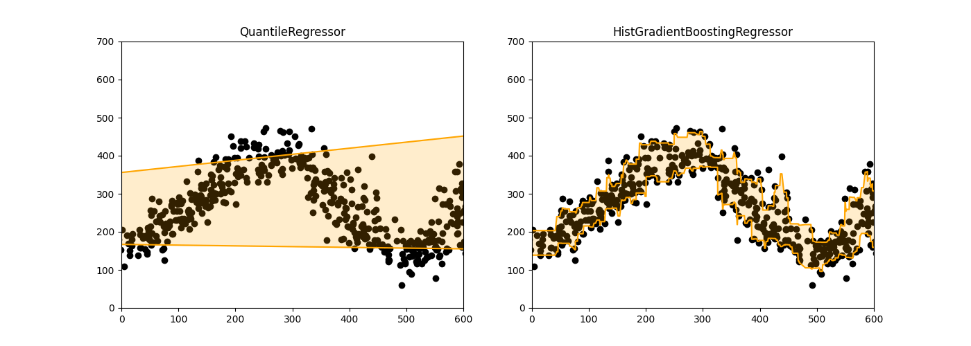
Random Forest for quantile regression
We can use even more complex models to derive the regression for our quantiles. The state of the art in random forest implementation with gradient boosting is HistGradientBoostingRegressor implemented in scikit-learn, which actually has the option to include the option ‘quantile’ as loss, which corresponds to the Pinball-loss we mentioned above. Then the option ‘quantile’ should determine the value of [math]\tau[/math].
5. Application to Reinforcement Learning
Q-learning and SARSA: In Reinforcement Learning we often use Temporal Difference (TD) learning methods and learn the optimal Q-values by minimising an MSE of the TDs. The temporal differences for off-policy Q-learning are defined as
[math]TD_Q = r(s,a) +\gamma \max_{\tilde{a}\in\mathcal{A}}Q(s’,\tilde{a}) – Q(s,a)[/math]
with [math]r[/math] the reward and [math]\gamma[/math] the discount factor. In standard Q-learning, the TDs are calculated assuming the optimal policy chooses the action with best Q for s’.
Another flavor is the SARSA policy, for which the TDs are defined for a specific sequence of [math](s,a,r,s’,a’)[/math], meaning that SARSA learns the Q-values which reproduce the behaviour policy. The next action [math]a'[/math] need not be in general the optimal one.
[math]TD_{SARSA} = r(s,a) +\gamma Q(s’,a’) – Q(s,a)[/math]
In both cases the Q-values are learned by minimising the MSE-loss,
[math]\min_{Q(s,a)}\frac{1}{2}|TD_{Q}|_2^2[/math] and [math]\min_{Q(s,a)}\frac{1}{2}|TD_{SARSA}|_2^2[/math]
Using stochastic gradient descent, for every sample [math](s,a,r,s’)[/math] or [math](s,a,r,s’,a’)[/math] we update the [math]Q(s,a)[/math] value iteratively
[math]Q(s,a) \leftarrow Q(s,a)+\lambda TD_{policy}(s,a,r,s'(,a’))[/math]
We apply online tabular Q-learning to learn the optimal policy in the FrozenLake environment of Gymnasium. Below the figure shows the convergence of the reward and episode lenght, as well as the training error. Interestingly, temporal differences are always positive in Q-learning because of the use of [math]\max_a Q(s’,a)[/math]. Similarly the SARSA method converges to the optimal policy, but the temporal differences are both positive and negative, and vary around zero.


There are cases when the maximum in the Q-learning update is taken over an estimated parameterized model, which may not be precise due to insufficient exploration. Another issue is that the estimation for some states and actions having not enough data could be unsafe. In such cases, we may want to avoid using maximum over parametrized models for Q-values and we try to stick to the available data. Then we can use as in Ref.[9] the expectile or percentile regression for our TD-error, choosing a very high value of [math]\tau[/math] — say 0.95 — in order to approximate the maximum.
Minimize Quantile TD-Loss
[math]\min_{Q(s,a)} PinballLoss^{\tau}(TD_{SARSA})=|\tau – 1_{\{TD_{SARSA}<0\}}||TD_{SARSA}| [/math]
Minimize Expectile TD-Loss
[math]\min_{Q(s,a)} L_2^{\tau}(TD_{SARSA})=|\tau – 1_{\{TD_{SARSA}<0\}}|TD_{SARSA}^2[/math]
The intuition is that we want to find the value [math]Q(s.a)[/math] equal to the highest possible sampled value of [math]r(s,a) + \gamma Q(s’,a’)[/math], which depends on the sampled [math](s’,a’)[/math] tuples.
Both versions converge in the online learning to the optimal policy. In both cases the temporal differences converge to negative values in their large majority (95%).


Cite as
@article{giovanidis2025_QER,
  title   = "Quantile and Expectile Regression",
  author  = "Giovanidis, Anastasios",
  journal = "anastasiosgiovanidis.net",
  year    = "2025",
  url     = "https://anastasiosgiovanidis.net/2025/01/07/quantile-expectile-regression/"
}
References
[1] https://github.com/probabl-ai/youtube-appendix/blob/main/02-quantile/notebook.ipynb and the YouTube video tutorial: https://www.youtube.com/watch?v=yLz1NELcIM0
[2] Expectile Regression Blog Medium: https://shorturl.at/yYqQk
[3] https://docs.scipy.org/doc/scipy/reference/generated/scipy.stats.expectile.html
[4] STAT 593 “Quantile regression” lecture slides by Joseph Salmon http://josephsalmon.eu
[5] Roger Koenker and Gilbert Basset, “Regression Quantiles” Econometrica, vol.46, no.1, 1978
[6] I. Takeuchi, Q.V. Le, T.D. Sears, and A.J. Smola. “Nonparametric Quantile Estimation”, Journal of Machine
Learning Research, 7:1231–1264, 2006
[7] Maxime Sangnier, Olivier Fercoq, Florence d’Alché-Buc, “Joint quantile regression in vector-valued RKHSs”, NIPS 2016
[8] Splines GAM introduction https://tesixiao.github.io/teaching/2022-winter-142a/pyGAM
[9] Ilya Kostrikov, Ashvin Nair, Sergey Levine, Offline Reinforcement Learning with Implicit Q-Learning, ICLR 2022